Cylindrical conformal map projection
 Mercator projection of the world between 85°S and 85°N. Note the size comparison of Greenland and Africa.
 The Mercator projection with
Tissot's indicatrix
of deformation.
The Mercator projection with
Tissot's indicatrix
of deformation.
 Mercator 1569 world map
(
Nova et Aucta Orbis Terrae Descriptio ad Usum Navigantium Emendate Accommodata
) showing latitudes 66°S to 80°N.
Mercator 1569 world map
(
Nova et Aucta Orbis Terrae Descriptio ad Usum Navigantium Emendate Accommodata
) showing latitudes 66°S to 80°N.
The
Mercator projection
(
) is a
conformal
cylindrical map projection
presented by
Flemish
geographer and cartographer
Gerardus Mercator
in 1569. It became the standard map projection for
navigation
due to its ability to represent north as 'up' and south as 'down' everywhere while preserving local directions and shapes. However, as a result, the Mercator projection inflates the size of objects the further they are from the equator. In a Mercator projection, landmasses such as
Greenland
and
Antarctica
appear far larger than they actually are relative to landmasses near the equator. Despite these drawbacks, the Mercator projection is well-suited to marine navigation and internet web maps and continues to be widely used today.
[1]
History
[
edit
]
There is some controversy over the origins of the Mercator. German
polymath
Erhard Etzlaub
engraved miniature "compass maps" (about 10×8 cm) of Europe and parts of Africa that spanned latitudes 0°?67° to allow adjustment of his portable pocket-size
sundials
. The projection found on these maps, dating to 1511, was stated by
John Snyder
in 1987 to be the same projection as Mercator's. However, given the geometry of a sundial, these maps may well have been based on the similar
central cylindrical projection
, a limiting case of the
gnomonic projection
, which is the basis for a sundial. Snyder amended his assessment to "a similar projection" in 1993.
Joseph Needham
, a historian of China, speculated that some
star charts
of the Chinese
Song Dynasty
may have been based on the Mercator projection;
[4]
however, this claim was presented without evidence, and astronomical historian Kazuhiko Miyajima concluded using cartometric analysis that these charts used an
equirectangular projection
instead.
[5]
Portuguese mathematician and cosmographer
Pedro Nunes
first described the mathematical principle of the loxodrome and its use in
marine navigation
. In 1537, he proposed constructing a nautical atlas composed of several large-scale sheets in the equirectangular projection as a way to minimize distortion of directions. If these sheets were brought to the same scale and assembled, they would approximate the Mercator projection.
In 1569, Gerhard Kremer, known by his trade name Gerardus Mercator, announced a new projection by publishing a large
planispheric
map measuring 202 by 124 cm (80 by 49 in) and printed in eighteen separate sheets. Mercator titled the map
Nova et Aucta Orbis Terrae Descriptio ad Usum Navigantium Emendata
: "A new and augmented description of Earth corrected for the use of sailors". This title, along with an elaborate explanation for using the projection that appears as a section of text on the map, shows that Mercator understood exactly what he had achieved and that he intended the projection to aid navigation. Mercator never explained the method of construction or how he arrived at it. Various hypotheses have been tendered over the years, but in any case Mercator's friendship with
Pedro Nunes
and his access to the loxodromic tables Nunes created likely aided his efforts.
English mathematician
Edward Wright
published the first accurate tables for constructing the projection in 1599 and, in more detail, in 1610, calling his treatise "Certaine Errors in Navigation". The first mathematical formulation was publicized around 1645 by a mathematician named Henry Bond (
c.
1600
?1678). However, the mathematics involved were developed but never published by mathematician
Thomas Harriot
starting around 1589.
The development of the Mercator projection represented a major breakthrough in the nautical cartography of the 16th century. However, it was much ahead of its time, since the old navigational and surveying techniques were not compatible with its use in navigation. Two main problems prevented its immediate application: the impossibility of determining the longitude at sea with adequate accuracy and the fact that
magnetic directions, instead of geographical directions
, were used in navigation. Only in the middle of the 18th century, after the
marine chronometer
was invented and the spatial distribution of
magnetic declination
was known, could the Mercator projection be fully adopted by navigators.
Despite those position-finding limitations, the Mercator projection can be found in many world maps in the centuries following Mercator's first publication. However, it did not begin to dominate world maps until the 19th century, when the problem of position determination had been largely solved. Once the Mercator became the usual projection for commercial and educational maps, it came under persistent criticism from cartographers for its unbalanced representation of landmasses and its inability to usefully show the polar regions.
The criticisms leveled against inappropriate use of the Mercator projection resulted in a flurry of new inventions in the late 19th and early 20th century, often directly touted as alternatives to the Mercator. Due to these pressures, publishers gradually reduced their use of the projection over the course of the 20th century. However, the advent of Web mapping gave the projection an abrupt resurgence in the form of the
Web Mercator projection
.
Today, the Mercator can be found in marine charts, occasional world maps, and Web mapping services, but commercial atlases have largely abandoned it, and wall maps of the world can be found in many alternative projections.
Google Maps
, which relied on it since 2005, still uses it for local-area maps but dropped the projection from desktop platforms in 2017 for maps that are zoomed out of local areas. Many other online mapping services still exclusively use the Web Mercator.
Properties
[
edit
]
 Comparison of tangent and secant forms of normal, oblique and transverse Mercator projections with standard parallels in red
As in all
cylindrical projections
,
parallels
and
meridians
on the Mercator are straight and perpendicular to each other. In accomplishing this, the unavoidable east?west stretching of the map, which increases as distance away from the
equator
increases, is accompanied in the Mercator projection by a corresponding north?south stretching, so that at every point location the east?west scale is the same as the north?south scale, making it a
conformal map projection
. Conformal projections preserve angles around all locations.
Because the linear scale of a Mercator map increases with latitude, it distorts the size of geographical objects far from the equator and conveys a distorted perception of the overall geometry of the planet. At latitudes greater than 70° north or south the Mercator projection is practically unusable, because the
linear scale
becomes infinitely large at the poles. A Mercator map can therefore never fully show the
polar areas
(as long as the projection is based on a cylinder centered on the Earth's rotation axis; see the
transverse Mercator projection
for another application).
The Mercator projection maps trajectories of constant
bearing
(called
rhumb lines
or
loxodromes
) to straight lines, and is thus uniquely suited to
marine navigation
: courses and bearings are measured using a
compass rose
or protractor, and the corresponding directions are easily transferred from point to point, on the map, e.g. with the help of a
parallel ruler
.
The Mercator projection is often compared to and confused with the
central cylindrical projection
, which is the result of projecting points from the sphere onto a tangent cylinder along straight radial lines, as if from a light source placed at the Earth's center.
[7]
Both have extreme distortion far from the equator and cannot show the poles. However, they are different projections and have different properties.
Distortion of sizes
[
edit
]
 Proportions of apparent size and real size (animated)
As on all
map projections
, shapes or sizes are distortions of the true layout of the Earth's surface.
The Mercator projection exaggerates areas far from the
equator
.
Examples of size distortion
[
edit
]
- Greenland
appears the same size as
Africa
, when in reality Africa's area is 14 times as large.
[8]
- Alaska
appears to be the same size as
Australia
, although Australia is actually 4.5 times as large.
- Alaska also takes as much area on the map as
Brazil
, whereas Brazil's area is nearly 5 times that of Alaska.
- Madagascar
and
Great Britain
look about the same size, while Madagascar is actually more than twice as large as Great Britain.
Criticism
[
edit
]
Because of great land area distortions, critics like George Kellaway and Irving Fisher consider the projection unsuitable for general world maps. Because it shows countries near the Equator as too small when compared to those of Europe and North America, it has been supposed
[
by whom?
]
to cause people to consider those countries as less important.
[9]
Mercator himself used the equal-area
sinusoidal projection
to show relative areas. However, despite such criticisms, the Mercator projection was, especially in the late 19th and early 20th centuries, perhaps the most common projection used in world maps.
[10]
[11]
[12]
Atlases
largely stopped using the Mercator projection for world maps or for areas distant from the equator in the 1940s, preferring other
cylindrical projections
, or forms of
equal-area projection
. The Mercator projection is, however, still commonly used for areas near the equator where distortion is minimal. It is also frequently found in maps of time zones.
Because of its common usage, the Mercator projection has been supposed
[
by whom?
]
to have influenced people's view of the world.
[14]
Arno Peters
stirred controversy beginning in 1972 when he proposed what is now usually called the
Gall?Peters projection
to remedy the problems of the Mercator, claiming it to be his own original work without referencing prior work by cartographers such as Gall's work from 1855. The projection he promoted is a specific parameterization of the
cylindrical equal-area projection
. In response, a 1989 resolution by seven North American geographical groups disparaged using cylindrical projections for general-purpose world maps, which would include both the Mercator and the Gall?Peters.
[15]
Uses
[
edit
]
Practically every marine chart in print is based on the Mercator projection due to its uniquely favorable properties for navigation. It is also commonly used by street map services hosted on the Internet, due to its uniquely favorable properties for local-area maps computed on demand.
[16]
Mercator projections were also important in the mathematical development of
plate tectonics
in the 1960s.
[17]
Marine navigation
[
edit
]
 A rhumb line (blue) compared to a great-circle arc (red) between Lisbon, Portugal, and Havana, Cuba. Top: orthographic projection. Bottom: Mercator projection.
The Mercator projection was designed for use in marine
navigation
because of its unique property of representing any course of constant
bearing
as a straight segment. Such a course, known as a
rhumb
(alternately called a rhumb line or loxodrome) is preferred in marine navigation because ships can sail in a constant compass direction. This reduces the difficult, error-prone course corrections that otherwise would be necessary when sailing a different course.
For small distances (compared to the radius of the Earth), the difference between the rhumb and the
great circle
course is negligible. Even for longer distances, the simplicity of the constant bearing makes it attractive. As observed by Mercator, on such a course, the ship would not arrive by the shortest route, but it will surely arrive. Sailing a rhumb meant that all that the sailors had to do was keep a constant course as long as they knew where they were when they started, where they intended to be when they finished, and had a map in Mercator projection that correctly showed those two coordinates.
Web Mercator
[
edit
]
Many major online street mapping services (
Bing Maps
,
Google Maps
,
Mapbox
,
MapQuest
,
OpenStreetMap
,
Yahoo! Maps
, and others) use a variant of the Mercator projection for their map images
[19]
called
Web Mercator
or Google Web Mercator. Despite its obvious scale variation at the world level (small scales), the projection is well-suited as an interactive world map that can be zoomed seamlessly to local (large-scale) maps, where there is relatively little distortion due to the variant projection's near-
conformality
.
The major online street mapping services' tiling systems display most of the world at the lowest zoom level as a single square image, excluding the polar regions by truncation at latitudes of
φ
max
= ±85.05113°. (See
below
.) Latitude values outside this range are mapped using a different relationship that does not diverge at
φ
= ±90°.
[
citation needed
]
Mathematics
[
edit
]
Cylindrical projections
[
edit
]
Although the surface of Earth is best modelled by an
oblate ellipsoid of revolution
, for
small scale
maps the ellipsoid is approximated by a sphere of radius
a
, where
a
is approximately 6,371 km. This spherical approximation of Earth can be modelled by a smaller sphere of radius
R
, called the
globe
in this section. The globe determines the scale of the map. The various
cylindrical projections
specify how the geographic detail is transferred from the globe to a cylinder tangential to it at the equator. The cylinder is then unrolled to give the planar map.
[
page needed
]
The fraction
R
/
a
is called the
representative fraction
(RF) or the
principal scale
of the projection. For example, a Mercator map printed in a book might have an equatorial width of 13.4 cm corresponding to a globe radius of 2.13 cm and an RF of approximately
1
/
300M
(M is used as an abbreviation for 1,000,000 in writing an RF) whereas Mercator's original 1569 map has a width of 198 cm corresponding to a globe radius of 31.5 cm and an RF of about
1
/
20M
.
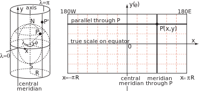
A cylindrical map projection is specified by formulae linking the geographic coordinates of latitude
φ
and longitude
λ
to Cartesian coordinates on the map with origin on the equator and
x
-axis along the equator. By construction, all points on the same meridian lie on the same
generator
[a]
of the cylinder at a constant value of
x
, but the distance
y
along the generator (measured from the equator) is an arbitrary
[b]
function of latitude,
y
(
φ
). In general this function does not describe the geometrical projection (as of light rays onto a screen) from the centre of the globe to the cylinder, which is only one of an unlimited number of ways to conceptually project a cylindrical map.
Since the cylinder is tangential to the globe at the equator, the
scale factor
between globe and cylinder is unity on the equator but nowhere else. In particular since the radius of a parallel, or circle of latitude, is
R
cos
φ
, the corresponding parallel on the map must have been stretched by a factor of
1
/
cos
φ
= sec
φ
. This scale factor on the parallel is conventionally denoted by
k
and the corresponding scale factor on the meridian is denoted by
h
.
[22]
Scale factor
[
edit
]
The Mercator projection is
conformal
. One implication of that is the "isotropy of scale factors", which means that the point scale factor is independent of direction, so that small shapes are preserved by the projection. This implies that the vertical scale factor,
h
, equals the horizontal scale factor,
k
. Since
k
=
sec
φ
, so must
h
.
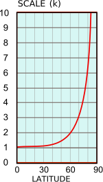
The graph shows the variation of this scale factor with latitude. Some numerical values are listed below.
- at latitude 30° the scale factor is
k
= sec 30° = 1.15,
- at latitude 45° the scale factor is
k
= sec 45° = 1.41,
- at latitude 60° the scale factor is
k
= sec 60° = 2,
- at latitude 80° the scale factor is
k
= sec 80° = 5.76,
- at latitude 85° the scale factor is
k
= sec 85° = 11.5
The area scale factor is the product of the parallel and meridian scales
hk
= sec
2
φ
. For Greenland, taking 73° as a median latitude,
hk
= 11.7. For Australia, taking 25° as a median latitude,
hk
= 1.2. For Great Britain, taking 55° as a median latitude,
hk
= 3.04.
The variation with latitude is sometimes indicated by multiple
bar scales
as shown below.

 Tissot's indicatrices
on the Mercator projection
Tissot's indicatrices
on the Mercator projection
The classic way of showing the distortion inherent in a projection is to use
Tissot's indicatrix
.
Nicolas Tissot
noted that the scale factors at a point on a map projection, specified by the numbers
h
and
k
, define an ellipse at that point. For cylindrical projections, the axes of the ellipse are aligned to the meridians and parallels.
[c]
For the Mercator projection,
h
=
k
, so the ellipses degenerate into circles with radius proportional to the value of the scale factor for that latitude. These circles are rendered on the projected map with extreme variation in size, indicative of Mercator's scale variations.
Mercator projection transformations
[
edit
]
Derivation
[
edit
]
As discussed above, the isotropy condition implies that
h
=
k
=
sec
φ
. Consider a point on the globe of radius
R
with longitude
λ
and latitude
φ
. If
φ
is increased by an infinitesimal amount,
dφ
, the point moves
R
dφ
along a meridian of the globe of radius
R
, so the corresponding change in
y
,
dy
, must be
hR
dφ
=
R
sec
φ
dφ
. Therefore
y′
(
φ
) =
R
sec
φ
. Similarly, increasing
λ
by
dλ
moves the point
R
cos
φ
dλ
along a parallel of the globe, so
dx
=
kR
cos
φ
dλ
=
R
dλ
. That is,
x′
(
λ
) =
R
. Integrating the equations

with
x
(
λ
0
) = 0 and
y
(0) = 0, gives
x(λ)
and
y(φ)
. The value
λ
0
is the longitude of an arbitrary central meridian that is usually, but not always,
that of Greenwich
(i.e., zero). The angles
λ
and
φ
are expressed in radians. By the
integral of the secant function
,
[24]
[25]

![{\displaystyle x=R(\lambda -\lambda _{0}),\qquad y=R\ln \left[\tan \left({\frac {\pi }{4}}+{\frac {\varphi }{2}}\right)\right].}](https://wikimedia.org/api/rest_v1/media/math/render/svg/62ea14e55f1e378a2a82a2ff70bee9d2f8cabf8d)
The function
y
(
φ
) is plotted alongside
φ
for the case
R
= 1: it tends to infinity at the poles. The linear
y
-axis values are not usually shown on printed maps; instead some maps show the non-linear scale of latitude values on the right. More often than not the maps show only a graticule of selected meridians and parallels.
Inverse transformations
[
edit
]
![{\displaystyle \lambda =\lambda _{0}+{\frac {x}{R}},\qquad \varphi =2\tan ^{-1}\left[\exp \left({\frac {y}{R}}\right)\right]-{\frac {\pi }{2}}\,.}](https://wikimedia.org/api/rest_v1/media/math/render/svg/adc1b673f6fcbd95688246bf8c30af7fdd9214ec)
The expression on the right of the second equation defines the
Gudermannian function
; i.e.,
φ
= gd(
y
/
R
): the direct equation may therefore be written as
y
=
R
·gd
?1
(
φ
).
[24]
Alternative expressions
[
edit
]
There are many alternative expressions for
y
(
φ
), all derived by elementary manipulations.
[25]
![{\displaystyle {\begin{aligned}y&=&{\frac {R}{2}}\ln \left[{\frac {1+\sin \varphi }{1-\sin \varphi }}\right]&=&{R}\ln \left[{\frac {1+\sin \varphi }{\cos \varphi }}\right]&=R\ln \left(\sec \varphi +\tan \varphi \right)\\[2ex]&=&R\tanh ^{-1}\left(\sin \varphi \right)&=&R\sinh ^{-1}\left(\tan \varphi \right)&=R\operatorname {sgn} (\varphi )\cosh ^{-1}\left(\sec \varphi \right)=R\operatorname {gd} ^{-1}(\varphi ).\end{aligned}}}](https://wikimedia.org/api/rest_v1/media/math/render/svg/ae347eb9bffadb5f8004faa0d0c1e212839b58a1)
Corresponding inverses are:

For angles expressed in degrees:
![{\displaystyle x={\frac {\pi R(\lambda ^{\circ }-\lambda _{0}^{\circ })}{180}},\qquad \quad y=R\ln \left[\tan \left(45+{\frac {\varphi ^{\circ }}{2}}\right)\right].}](https://wikimedia.org/api/rest_v1/media/math/render/svg/dcc9392cd18cd854770761b77b8d37a0633c1354)
The above formulae are written in terms of the globe radius
R
. It is often convenient to work directly with the map width
W
= 2
π
R
. For example, the basic transformation equations become
![{\displaystyle x={\frac {W}{2\pi }}\left(\lambda -\lambda _{0}\right),\qquad \quad y={\frac {W}{2\pi }}\ln \left[\tan \left({\frac {\pi }{4}}+{\frac {\varphi }{2}}\right)\right].}](https://wikimedia.org/api/rest_v1/media/math/render/svg/a7abeaed8bf4f766e4eb931035dfbbf787caa6c0)
Truncation and aspect ratio
[
edit
]
The ordinate
y
of the Mercator projection becomes infinite at the poles and the map must be truncated at some latitude less than ninety degrees. This need not be done symmetrically. Mercator's original map is truncated at 80°N and 66°S with the result that European countries were moved toward the centre of the map. The
aspect ratio
of his map is
198
/
120
= 1.65. Even more extreme truncations have been used: a
Finnish school atlas
was truncated at approximately 76°N and 56°S, an aspect ratio of 1.97.
Much Web-based mapping uses a zoomable version of the Mercator projection with an aspect ratio of one. In this case the maximum latitude attained must correspond to
y
= ±
W
/
2
, or equivalently
y
/
R
=
π
. Any of the inverse transformation formulae may be used to calculate the corresponding latitudes:
![{\displaystyle \varphi =\tan ^{-1}\left[\sinh \left({\frac {y}{R}}\right)\right]=\tan ^{-1}\left[\sinh \pi \right]=\tan ^{-1}\left[11.5487\right]=85.05113^{\circ }.}](https://wikimedia.org/api/rest_v1/media/math/render/svg/0e455a07f94771d84de1d2c0de4e0ed371c3858c)
Small element geometry
[
edit
]
The relations between
y
(
φ
) and properties of the projection, such as the transformation of angles and the variation in scale, follow from the geometry of corresponding
small
elements on the globe and map. The figure below shows a point P at latitude
φ
and longitude
λ
on the globe and a nearby point Q at latitude
φ
+
δφ
and longitude
λ
+
δλ
. The vertical lines PK and MQ are arcs of meridians of length
Rδφ
.
[d]
The horizontal lines PM and KQ are arcs of parallels of length
R
(cos
φ
)
δλ
. The corresponding points on the projection define a rectangle of width
δx
and height
δy
.

For small elements, the angle PKQ is approximately a right angle and therefore

The previously mentioned scaling factors from globe to cylinder are given by
- parallel scale factor

- meridian scale factor

Since the meridians are mapped to lines of constant
x
, we must have
x
=
R
(
λ
?
λ
0
)
and
δx
=
Rδλ
, (
λ
in radians). Therefore, in the limit of infinitesimally small elements

In the case of the Mercator projection,
y'
(
φ
) =
R
sec
φ
, so this gives us
h
=
k
and
α
=
β
. The fact that
h
=
k
is the isotropy of scale factors discussed above. The fact that
α
=
β
reflects another implication of the mapping being conformal, namely the fact that a sailing course of constant azimuth on the globe is mapped into the same constant grid bearing on the map.
Formulae for distance
[
edit
]
Converting ruler distance on the Mercator map into true (
great circle
) distance on the sphere is straightforward along the equator but nowhere else. One problem is the variation of scale with latitude, and another is that straight lines on the map (
rhumb lines
), other than the meridians or the equator, do not correspond to great circles.
The distinction between rhumb (sailing) distance and great circle (true) distance was clearly understood by Mercator. (See
Legend 12
on the 1569 map.) He stressed that the rhumb line distance is an acceptable approximation for true great circle distance for courses of short or moderate distance, particularly at lower latitudes. He even quantifies his statement: "When the great circle distances which are to be measured in the vicinity of the equator do not exceed 20 degrees of a great circle, or 15 degrees near Spain and France, or 8 and even 10 degrees in northern parts it is convenient to use rhumb line distances".
For a ruler measurement of a
short
line, with midpoint at latitude
φ
, where the scale factor is
k
= sec
φ
=
1
/
cos
φ
:
- True distance = rhumb distance ? ruler distance × cos
φ
/ RF. (short lines)
With radius and great circle circumference equal to 6,371 km and 40,030 km respectively an RF of
1
/
300M
, for which
R
= 2.12 cm and
W
= 13.34 cm, implies that a ruler measurement of 3 mm. in any direction from a point on the equator corresponds to approximately 900 km. The corresponding distances for latitudes 20°, 40°, 60° and 80° are 846 km, 689 km, 450 km and 156 km respectively.
Longer distances require various approaches.
On the equator
[
edit
]
Scale is unity on the equator (for a non-secant projection). Therefore, interpreting ruler measurements on the equator is simple:
- True distance = ruler distance / RF (equator)
For the above model, with RF =
1
/
300M
, 1 cm corresponds to 3,000 km.
On other parallels
[
edit
]
On any other parallel the scale factor is sec
φ
so that
- Parallel distance = ruler distance × cos
φ
/ RF (parallel).
For the above model 1 cm corresponds to 1,500 km at a latitude of 60°.
This is not the shortest distance between the chosen endpoints on the parallel because a parallel is not a great circle. The difference is small for short distances but increases as
λ
, the longitudinal separation, increases. For two points, A and B, separated by 10° of longitude on the parallel at 60° the distance along the parallel is approximately 0.5 km greater than the great circle distance. (The distance AB along the parallel is (
a
cos
φ
)
λ
. The length of the chord AB is 2(
a
cos
φ
) sin
λ
/
2
. This chord subtends an angle at the centre equal to 2arcsin(cos
φ
sin
λ
/
2
) and the great circle distance between A and B is 2
a
arcsin(cos
φ
sin
λ
/
2
).) In the extreme case where the longitudinal separation is 180°, the distance along the parallel is one half of the circumference of that parallel; i.e., 10,007.5 km. On the other hand, the
geodesic
between these points is a great circle arc through the pole subtending an angle of 60° at the center: the length of this arc is one sixth of the great circle circumference, about 6,672 km. The difference is 3,338 km so the ruler distance measured from the map is quite misleading even after correcting for the latitude variation of the scale factor.
On a meridian
[
edit
]
A meridian of the map is a great circle on the globe but the continuous scale variation means ruler measurement alone cannot yield the true distance between distant points on the meridian. However, if the map is marked with an accurate and finely spaced latitude scale from which the latitude may be read directly?as is the case for the
Mercator 1569 world map
(sheets 3, 9, 15) and all subsequent nautical charts?the meridian distance between two latitudes
φ
1
and
φ
2
is simply

If the latitudes of the end points cannot be determined with confidence then they can be found instead by calculation on the ruler distance. Calling the ruler distances of the end points on the map meridian as measured from the equator
y
1
and
y
2
, the true distance between these points on the sphere is given by using any one of the inverse Mercator formulæ:
![{\displaystyle m_{12}=a\left|\tan ^{-1}\left[\sinh \left({\frac {y_{1}}{R}}\right)\right]-\tan ^{-1}\left[\sinh \left({\frac {y_{2}}{R}}\right)\right]\right|,}](https://wikimedia.org/api/rest_v1/media/math/render/svg/47121a7581ab0e8d755c23df8ac6708bfe8d57c4)
where
R
may be calculated from the width
W
of the map by
R
=
W
/
2
π
. For example, on a map with
R
= 1 the values of
y
= 0, 1, 2, 3 correspond to latitudes of
φ
= 0°, 50°, 75°, 84° and therefore the successive intervals of 1 cm on the map correspond to latitude intervals on the globe of 50°, 25°, 9° and distances of 5,560 km, 2,780 km, and 1,000 km on the Earth.
On a rhumb
[
edit
]
A straight line on the Mercator map at angle
α
to the meridians is a
rhumb line
. When
α
=
π
/
2
or
3
π
/
2
the rhumb corresponds to one of the parallels; only one, the equator, is a great circle. When
α
= 0 or
π
it corresponds to a meridian great circle (if continued around the Earth). For all other values it is a spiral from pole to pole on the globe intersecting all meridians at the same angle, and is thus not a great circle.
[25]
This section discusses only the last of these cases.
If
α
is neither 0 nor
π
then the
above figure
of the infinitesimal elements shows that the length of an infinitesimal rhumb line on the sphere between latitudes
φ
; and
φ
+
δφ
is
a
sec
α
δφ
. Since
α
is constant on the rhumb this expression can be integrated to give, for finite rhumb lines on the Earth:

Once again, if Δ
φ
may be read directly from an accurate latitude scale on the map, then the rhumb distance between map points with latitudes
φ
1
and
φ
2
is given by the above. If there is no such scale then the ruler distances between the end points and the equator,
y
1
and
y
2
, give the result via an inverse formula:

These formulæ give rhumb distances on the sphere which may differ greatly from true distances whose determination requires more sophisticated calculations.
[e]
Generalization to the ellipsoid
[
edit
]
When the Earth is modelled by a
spheroid
(
ellipsoid
of revolution) the Mercator projection must be modified if it is to remain
conformal
. The transformation equations and scale factor for the non-secant version are
[26]
![{\displaystyle {\begin{aligned}x&=R\left(\lambda -\lambda _{0}\right),\\y&=R\ln \left[\tan \left({\frac {\pi }{4}}+{\frac {\varphi }{2}}\right)\left({\frac {1-e\sin \varphi }{1+e\sin \varphi }}\right)^{\frac {e}{2}}\right]=R\left(\sinh ^{-1}\left(\tan \varphi \right)-e\tanh ^{-1}(e\sin \varphi )\right),\\k&=\sec \varphi {\sqrt {1-e^{2}\sin ^{2}\varphi }}.\end{aligned}}}](https://wikimedia.org/api/rest_v1/media/math/render/svg/378a7fde0b2ede2f7f7b1b663f9e00c5aa34cea9)
The scale factor is unity on the equator, as it must be since the cylinder is tangential to the ellipsoid at the equator. The ellipsoidal correction of the scale factor increases with latitude but it is never greater than
e
2
, a correction of less than 1%. (The value of
e
2
is about 0.006 for all reference ellipsoids.) This is much smaller than the scale inaccuracy, except very close to the equator. Only accurate Mercator projections of regions near the equator will necessitate the ellipsoidal corrections.
The inverse is solved iteratively, as the
isometric latitude
is involved.
See also
[
edit
]
Notes
[
edit
]
- ^
A generator of a cylinder is a straight line on the surface parallel to the axis of the cylinder.
- ^
The function
y
(
φ
) is not completely arbitrary: it must be monotonic increasing and antisymmetric (
y
(?
φ
) = ?
y
(
φ
), so that
y
(0)=0): it is normally continuous with a continuous first derivative.
- ^
More general example of Tissot's indicatrix: the
Winkel tripel
projection.
- ^
R
is the radius of the globe.
- ^
See
great-circle distance
, the
Vincenty's formulae
, or
Mathworld
.
References
[
edit
]
- ^
"Gerardus Mercator"
.
education.nationalgeographic.org
. Retrieved
2024-03-02
.
- ^
Needham, Joseph (1959).
Science and Civilization in China
. Vol. 3. Cambridge University Press. pp. 277, 545.
- ^
Miyajima, Kazuhiko (1998).
"Projection Methods in Chinese, Korean and Japanese Star Maps"
.
Highlights of Astronomy
.
11
(2): 712?715.
doi
:
10.1017/s1539299600018554
.
- ^
Frederick Rickey, V.; Tuchinsky, Philip M. (May 1980).
"An application of geography to mathematics: history of the integral of the secant"
.
Mathematics Magazine
.
53
(3): 164.
doi
:
10.2307/2690106
. Retrieved
18 August
2022
.
- ^
"This animated map shows the true size of each country"
.
Nature Index
. 2019-08-27
. Retrieved
2023-06-20
.
- ^
"Mercator Projection vs. Peters Projection, part 1"
. Matt T. Rosenberg, about.com.
- ^
Kellaway, G.P. (1946).
Map Projections
p. 37?38. London: Methuen & Co. LTD. (According to this source, it had been claimed that the Mercator projection was used for "imperialistic motives")
- ^
Abelson, C.E. (1954).
Common Map Projections
s. 4. Sevenoaks: W.H. Smith & Sons.
- ^
Chamberlin, Wellman (1947).
The Round Earth on Flat Paper
s. 99. Washington, D.C.: The National Geographic Society.
- ^
"Mercator Projection vs. Peters Projection, part 2"
. Matt T. Rosenberg, about.com.
- ^
American Cartographer. 1989. 16(3): 222?223.
- ^
[1]
[
self-published source
]
- ^
Cox, Allan, ed. (1973).
Plate Tectonics and Geomagnetic Reversals
. W.H. Freeman. p. 46.
- ^
Battersby, Sarah E.; Finn, Michael P.; Usery, E. Lynn; Yamamoto, Kristina H. (June 1, 2014).
"Implications of Web Mercator and Its Use in Online Mapping"
.
Cartographica: The International Journal for Geographic Information and Geovisualization
.
49
(2): 85?101.
doi
:
10.3138/carto.49.2.2313
.
ISSN
0317-7173
.
- ^
Snyder.
Working Manual, page 20.
- ^
a
b
NIST.
See Sections
4.26#ii
and
4.23#viii
- ^
a
b
c
Osborne 2013
, Chapter 2
- ^
Osborne 2013
, Chapters 5, 6
Bibliography
[
edit
]
- Maling, Derek Hylton (1992),
Coordinate Systems and Map Projections
(second ed.), Pergamon Press,
ISBN
0-08-037233-3
.
- Monmonier, Mark
(2004),
Rhumb Lines and Map Wars: A Social History of the Mercator Projection
(Hardcover ed.), Chicago: The University of Chicago Press,
ISBN
0-226-53431-6
- Olver, F. W.J.; Lozier, D.W.; Boisvert, R.F.; et al., eds. (2010),
NIST Handbook of Mathematical Functions
, Cambridge University Press
- Osborne, Peter (14 November 2013),
The Mercator Projections
,
doi
:
10.5281/zenodo.35392
(Supplements:
Maxima files
and
Latex code and figures
)
- Snyder, John P
(1993),
Flattening the Earth: Two Thousand Years of Map Projections
, University of Chicago Press,
ISBN
0-226-76747-7
- Snyder, John P. (1987),
Map Projections ? A Working Manual. U.S. Geological Survey Professional Paper 1395
, United States Government Printing Office, Washington, D.C.
This paper can be downloaded from
USGS pages.
It gives full details of most projections, together with interesting introductory sections, but it does not derive any of the projections from first principles.
Further reading
[
edit
]
- Rapp, Richard H (1991),
Geometric Geodesy, Part I
, Ohio State University Department of Geodetic Science and Surveying,
hdl
:
1811/24333
External links
[
edit
]
|
|---|
| International
| |
|---|
| National
| |
|---|
| Other
| |
|---|