Azimuthal equal-area map projection
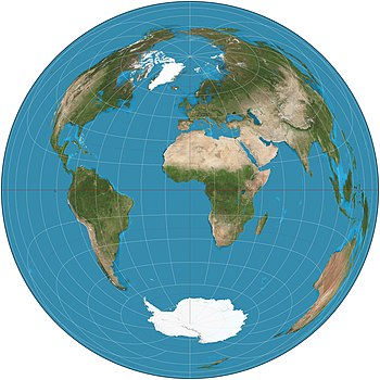 Lambert azimuthal equal-area projection of the world. The center is 0° N 0° E. The antipode is 0° N 180° E, near
Kiribati
in the
Pacific Ocean
. That point is represented by the entire circular boundary of the map, and the ocean around that point appears along the entire boundary.
Lambert azimuthal equal-area projection of the world. The center is 0° N 0° E. The antipode is 0° N 180° E, near
Kiribati
in the
Pacific Ocean
. That point is represented by the entire circular boundary of the map, and the ocean around that point appears along the entire boundary.
 The Lambert azimuthal equal-area projection with
Tissot's indicatrix
of deformation.
The Lambert azimuthal equal-area projection with
Tissot's indicatrix
of deformation.
The
Lambert azimuthal equal-area projection
is a particular mapping from a sphere to a
disk
. It accurately represents
area
in all regions of the sphere, but it does not accurately represent
angles
. It is named for the
Swiss
mathematician
Johann Heinrich Lambert
, who announced it in 1772.
[1]
"Zenithal" being synonymous with "azimuthal", the projection is also known as the
Lambert zenithal equal-area projection
.
[2]
The Lambert azimuthal projection is used as a
map projection
in
cartography
. For example, the
National Atlas of the US
uses a Lambert azimuthal equal-area projection to display information in the online Map Maker application,
[3]
and the
European Environment Agency
recommends its usage for European mapping for statistical analysis and display.
[4]
It is also used in scientific disciplines such as
geology
for plotting the orientations of lines in three-dimensional space. This plotting is aided by a special kind of
graph paper
called a
Schmidt net
.
[5]
Definition
[
edit
]
 A
cross sectional
view of the sphere and a plane tangent to it at
S
. Each point on the sphere (except the antipode) is projected to the plane along a circular arc centered at the point of tangency between the sphere and plane.
A
cross sectional
view of the sphere and a plane tangent to it at
S
. Each point on the sphere (except the antipode) is projected to the plane along a circular arc centered at the point of tangency between the sphere and plane.
To define the Lambert azimuthal projection, imagine a plane set tangent to the sphere at some point
S
on the sphere. Let
P
be any point on the sphere other than the
antipode
of
S
. Let
d
be the distance between
S
and
P
in three-dimensional space (
not
the distance along the sphere surface). Then the projection sends
P
to a point
P′
on the plane that is a distance
d
from
S
.
To make this more precise, there is a unique circle centered at
S
, passing through
P
, and perpendicular to the plane. It intersects the plane in two points; let
P
′ be the one that is closer to
P
. This is the projected point. See the figure. The antipode of
S
is excluded from the projection because the required circle is not unique. The case of
S
is degenerate;
S
is projected to itself, along a circle of radius 0.
[6]
Explicit formulas are required for carrying out the projection on a
computer
. Consider the projection centered at
S
= (0, 0, ?1)
on the
unit sphere
, which is the set of points
(
x
,
y
,
z
)
in three-dimensional space
R
3
such that
x
2
+
y
2
+
z
2
= 1
. In
Cartesian coordinates
(
x
,
y
,
z
)
on the sphere and
(
X
,
Y
)
on the plane, the projection and its inverse are then described by

In
spherical coordinates
(
ψ
,
θ
)
on the sphere (with
ψ
the
colatitude
and
θ
the longitude) and
polar coordinates
(
R
,
Θ
)
on the disk, the map and its inverse are given by
[6]

In
cylindrical coordinates
(
r
,
θ
,
z
)
on the sphere and polar coordinates
(
R
,
Θ
)
on the plane, the map and its inverse are given by

The projection can be centered at other points, and defined on spheres of radius other than 1, using similar formulas.
[7]
Properties
[
edit
]
As defined in the preceding section, the Lambert azimuthal projection of the unit sphere is undefined at (0, 0, 1). It sends the rest of the sphere to the open disk of radius 2 centered at the origin (0, 0) in the plane. It sends the point (0, 0, ?1) to (0, 0), the equator
z
= 0 to the circle of radius
√
2
centered at (0, 0), and the lower hemisphere
z
< 0 to the open disk contained in that circle.
The projection is a
diffeomorphism
(a
bijection
that is
infinitely differentiable
in both directions) between the sphere (minus (0, 0, 1)) and the open disk of radius 2. It is an area-preserving (equal-area) map, which can be seen by computing the
area element
of the sphere when parametrized by the inverse of the projection. In Cartesian coordinates it is

This means that measuring the area of a region on the sphere is tantamount to measuring the area of the corresponding region on the disk.
On the other hand, the projection does not preserve angular relationships among curves on the sphere. No mapping between a portion of a sphere and the plane can preserve both angles and areas. (If one did, then it would be a local
isometry
and would preserve
Gaussian curvature
; but the sphere and disk have different curvatures, so this is impossible.) This fact, that flat pictures cannot perfectly represent regions of spheres, is the fundamental problem of cartography.
As a consequence, regions on the sphere may be projected to the plane with greatly distorted shapes. This distortion is particularly dramatic far away from the center of the projection (0, 0, ?1). In practice the projection is often restricted to the hemisphere centered at that point; the other hemisphere can be mapped separately, using a second projection centered at the antipode.
Applications
[
edit
]
The Lambert azimuthal projection was originally conceived as an equal-area map projection. It is now also used in disciplines such as
geology
to plot directional data, as follows.
A direction in three-dimensional space corresponds to a line through the origin. The set of all such lines is itself a space, called the
real projective plane
in
mathematics
. Every line through the origin intersects the unit sphere in exactly two points, one of which is on the lower hemisphere
z
≤ 0. (Horizontal lines intersect the equator
z
= 0 in two antipodal points. It is understood that antipodal points on the equator represent a single line. See
quotient topology
.) Hence the directions in three-dimensional space correspond (almost perfectly) to points on the lower hemisphere. The hemisphere can then be plotted as a disk of radius
√
2
using the Lambert azimuthal projection.
Thus the Lambert azimuthal projection lets us plot directions as points in a disk. Due to the equal-area property of the projection, one can
integrate
over regions of the real projective plane (the space of directions) by integrating over the corresponding regions on the disk. This is useful for statistical analysis of directional data,
[6]
including random rigid
rotation
.
[8]
Not only lines but also planes through the origin can be plotted with the Lambert azimuthal projection. A plane intersects the hemisphere in a circular arc, called the
trace
of the plane, which projects down to a curve (typically non-circular) in the disk. One can plot this curve, or one can alternatively replace the plane with the line perpendicular to it, called the
pole
, and plot that line instead. When many planes are being plotted together, plotting poles instead of traces produces a less cluttered plot.
Researchers in
structural geology
use the Lambert azimuthal projection to plot
crystallographic
axes and faces,
lineation
and
foliation
in rocks,
slickensides
in
faults
, and other linear and planar features. In this context the projection is called the
equal-area hemispherical projection
. There is also an equal-angle hemispherical projection defined by
stereographic projection
.
[6]
The discussion here has emphasized an inside-out view of the lower hemisphere
z
≤ 0 (as might be seen in a star chart), but some disciplines (such as cartography) prefer an outside-in view of the upper hemisphere
z
≥ 0.
[6]
Indeed, any hemisphere can be used to record the lines through the origin in three-dimensional space.
Comparison of the
Lambert azimuthal equal-area projection
and some azimuthal projections centred on 90° N at the same scale, ordered by projection altitude in Earth radii.
(click for detail)
Animated Lambert projection
[
edit
]
[
citation needed
]
 Animation of a Lambert projection. Each grid cell maintains its area throughout the transformation. In this animation, points on the equator remain always on the
 plane.
 In this animated Lambert projection, the south pole is held fixed.
Let
 be two parameters for which
 and
and
 . Let
. Let
 be a "time" parameter (equal to the height, or vertical thickness, of the shell in the animation). If a uniform rectilinear grid is drawn in
space, then any point in this grid is transformed to a point
be a "time" parameter (equal to the height, or vertical thickness, of the shell in the animation). If a uniform rectilinear grid is drawn in
space, then any point in this grid is transformed to a point
 on a spherical shell of height
according to the mapping
on a spherical shell of height
according to the mapping


where
![{\displaystyle \lambda (u,H)={\frac {1}{2}}{\sqrt {(1-u)\left[8-H^{2}(1-u)\right]}}}](https://wikimedia.org/api/rest_v1/media/math/render/svg/4cf3eaae0a7651d0fcc7f6b38101f8c6848b7ad8) . Each frame in the animation corresponds to a parametric plot of the deformed grid at a fixed value of the shell height
(ranging from 0 to 2). Physically,
. Each frame in the animation corresponds to a parametric plot of the deformed grid at a fixed value of the shell height
(ranging from 0 to 2). Physically,
 is the stretch (deformed length divided by initial length) of infinitesimal line
 line segments. This mapping can be converted to one that keeps the south pole fixed by instead using

Regardless of the values of
 , the Jacobian of this mapping is everywhere equal to 1, showing that it is indeed an equal area mapping throughout the animation. This generalized mapping includes the Lambert projection as a special case when
 .
.
Application: this mapping can assist in explaining the meaning of a Lambert projection by showing it to "peel open" the sphere at a pole, morphing it to a disk without changing area enclosed by grid cells.
See also
[
edit
]
References
[
edit
]
- ^
Mulcahy, Karen.
"Lambert Azimuthal Equal Area"
.
City University of New York
. Retrieved
2007-03-30
.
- ^
The Times Atlas of the World
(1967), Boston: Houghton Mifflin, Plate 3, et passim.
- ^
"Map Projections: From Spherical Earth to Flat Map"
.
United States Department of the Interior
. 2008-04-29. Archived from
the original
on 2009-05-07
. Retrieved
2009-04-08
.
- ^
"Short Proceedings of the 1st European Workshop on Reference Grids, Ispra, 27-29 October 2003"
(PDF)
.
European Environment Agency
. 2004-06-14. p. 6
. Retrieved
2009-08-27
.
- ^
Ramsay (1967)
- ^
a
b
c
d
e
Borradaile (2003).
- ^
"Geomatics Guidance Note 7, part 2: Coordinate Conversions & Transformations including Formulas"
(PDF)
.
International Association of Oil & Gas Producers
. September 2016
. Retrieved
2017-12-17
.
- ^
Brannon, R.M.,
"Rotation, Reflection, and Frame Change"
, 2018
Sources
[
edit
]
- Borradaile, Graham J. (2003).
Statistics of Earth science data
. Berlin: Springer-Verlag.
ISBN
3-540-43603-0
.
- Do Carmo
; Manfredo P. (1976).
Differential geometry of curves and surfaces
. Englewood Cliffs, New Jersey: Prentice Hall.
ISBN
0-13-212589-7
.
- Hobbs, Bruce E., Means, Winthrop D., and Williams, Paul F. (1976).
An outline of structural geology
. New York: John Wiley & Sons, Inc.
ISBN
0-471-40156-0
.
{{
cite book
}}
: CS1 maint: multiple names: authors list (
link
)
- Ramsay, John G. (1967).
Folding and fracturing of rocks
. New York: McGraw-Hill.
- Spivak, Michael (1999).
A comprehensive introduction to differential geometry
. Houston, Texas: Publish or Perish.
ISBN
0-914098-70-5
.
External links
[
edit
]