Technique for dimensionality reduction
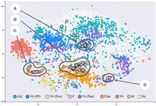 T-SNE visualisation of
word embeddings
generated using 19th century literature
T-SNE visualisation of
word embeddings
generated using 19th century literature
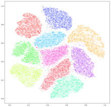 T-SNE embeddings of
MNIST
dataset
T-SNE embeddings of
MNIST
dataset
t-distributed stochastic neighbor embedding
(
t-SNE
) is a
statistical
method for visualizing high-dimensional data by giving each datapoint a location in a two or three-dimensional map. It is based on Stochastic Neighbor Embedding originally developed by
Geoffrey Hinton
and Sam Roweis,
[1]
where Laurens van der Maaten proposed the
t
-distributed
variant.
[2]
It is a
nonlinear dimensionality reduction
technique for embedding high-dimensional data for visualization in a low-dimensional space of two or three dimensions. Specifically, it models each high-dimensional object by a two- or three-dimensional point in such a way that similar objects are modeled by nearby points and dissimilar objects are modeled by distant points with high probability.
The t-SNE algorithm comprises two main stages. First, t-SNE constructs a
probability distribution
over pairs of high-dimensional objects in such a way that similar objects are assigned a higher probability while dissimilar points are assigned a lower probability. Second, t-SNE defines a similar probability distribution over the points in the low-dimensional map, and it minimizes the
Kullback?Leibler divergence
(KL divergence) between the two distributions with respect to the locations of the points in the map. While the original algorithm uses the
Euclidean distance
between objects as the base of its similarity metric, this can be changed as appropriate. A
Riemannian
variant is
UMAP
.
t-SNE has been used for visualization in a wide range of applications, including
genomics
,
computer security
research,
[3]
natural language processing
,
music analysis
,
[4]
cancer research
,
[5]
bioinformatics
,
[6]
geological domain interpretation,
[7]
[8]
[9]
and biomedical signal processing.
[10]
While t-SNE plots often seem to display
clusters
, the visual clusters can be influenced strongly by the chosen parameterization and therefore a good understanding of the parameters for t-SNE is necessary. Such "clusters" can be shown to even appear in non-clustered data,
[11]
and thus may be false findings. Interactive exploration may thus be necessary to choose parameters and validate results.
[12]
[13]
It has been demonstrated that t-SNE is often able to recover well-separated clusters, and with special parameter choices, approximates a simple form of
spectral clustering
.
[14]
For a data set with
n
elements, t-SNE runs in
O(
n
2
)
time and requires
O(
n
2
)
space.
[15]
Details
[
edit
]
Given a set of
 high-dimensional objects
 , t-SNE first computes probabilities
 that are proportional to the similarity of objects
 and
and
 , as follows.
For
 , define

and set
 .
Note the above denominator ensures
.
Note the above denominator ensures
 for all
 .
.
As van der Maaten and Hinton explained: "The similarity of datapoint
 to datapoint
 is the conditional probability,
 , that
would pick
as its neighbor if neighbors were picked in proportion to their probability density under a Gaussian centered at
."
[2]
, that
would pick
as its neighbor if neighbors were picked in proportion to their probability density under a Gaussian centered at
."
[2]
Now define

This is motivated because
 and
and
 from the N samples are estimated as 1/N, so the conditional probability can be written as
 and
and
 . Since
 , you can obtain previous formula.
Also note that
 and
and
 .
.
The bandwidth of the
Gaussian kernels
 is set in such a way that the
entropy
of the conditional distribution equals a predefined entropy using the
bisection method
. As a result, the bandwidth is adapted to the
density
of the data: smaller values of
are used in denser parts of the data space.
is set in such a way that the
entropy
of the conditional distribution equals a predefined entropy using the
bisection method
. As a result, the bandwidth is adapted to the
density
of the data: smaller values of
are used in denser parts of the data space.
Since the Gaussian kernel uses the Euclidean distance
 , it is affected by the
curse of dimensionality
, and in high dimensional data when distances lose the ability to discriminate, the
become too similar (asymptotically, they would converge to a constant). It has been proposed to adjust the distances with a power transform, based on the
intrinsic dimension
of each point, to alleviate this.
[16]
, it is affected by the
curse of dimensionality
, and in high dimensional data when distances lose the ability to discriminate, the
become too similar (asymptotically, they would converge to a constant). It has been proposed to adjust the distances with a power transform, based on the
intrinsic dimension
of each point, to alleviate this.
[16]
t-SNE aims to learn a
 -dimensional map
 (with
(with
 and
typically chosen as 2 or 3) that reflects the similarities
as well as possible. To this end, it measures similarities
and
typically chosen as 2 or 3) that reflects the similarities
as well as possible. To this end, it measures similarities
 between two points in the map
 and
and
 , using a very similar approach.
Specifically, for
, define
as
, using a very similar approach.
Specifically, for
, define
as

and set
 .
Herein a heavy-tailed
Student t-distribution
(with one-degree of freedom, which is the same as a
Cauchy distribution
) is used to measure similarities between low-dimensional points in order to allow dissimilar objects to be modeled far apart in the map.
.
Herein a heavy-tailed
Student t-distribution
(with one-degree of freedom, which is the same as a
Cauchy distribution
) is used to measure similarities between low-dimensional points in order to allow dissimilar objects to be modeled far apart in the map.
The locations of the points
in the map are determined by minimizing the (non-symmetric)
Kullback?Leibler divergence
of the distribution
 from the distribution
 , that is:

The minimization of the Kullback?Leibler divergence with respect to the points
is performed using
gradient descent
.
The result of this optimization is a map that reflects the similarities between the high-dimensional inputs.
Software
[
edit
]
- The R package
Rtsne
implements t-SNE in
R
.
- ELKI
contains tSNE, also with Barnes-Hut approximation
- scikit-learn
, a popular machine learning library in Python implements t-SNE with both exact solutions and the Barnes-Hut approximation.
- Tensorboard, the visualization kit associated with
TensorFlow
, also implements t-SNE (
online version
)
References
[
edit
]
- ^
Hinton, Geoffrey; Roweis, Sam (January 2002).
Stochastic neighbor embedding
(PDF)
.
Neural Information Processing Systems
.
- ^
a
b
van der Maaten, L.J.P.; Hinton, G.E. (Nov 2008).
"Visualizing Data Using t-SNE"
(PDF)
.
Journal of Machine Learning Research
.
9
: 2579?2605.
- ^
Gashi, I.; Stankovic, V.; Leita, C.; Thonnard, O. (2009). "An Experimental Study of Diversity with Off-the-shelf AntiVirus Engines".
Proceedings of the IEEE International Symposium on Network Computing and Applications
: 4?11.
- ^
Hamel, P.; Eck, D. (2010). "Learning Features from Music Audio with Deep Belief Networks".
Proceedings of the International Society for Music Information Retrieval Conference
: 339?344.
- ^
Jamieson, A.R.; Giger, M.L.; Drukker, K.; Lui, H.; Yuan, Y.; Bhooshan, N. (2010).
"Exploring Nonlinear Feature Space Dimension Reduction and Data Representation in Breast CADx with Laplacian Eigenmaps and t-SNE"
.
Medical Physics
.
37
(1): 339?351.
doi
:
10.1118/1.3267037
.
PMC
2807447
.
PMID
20175497
.
- ^
Wallach, I.; Liliean, R. (2009).
"The Protein-Small-Molecule Database, A Non-Redundant Structural Resource for the Analysis of Protein-Ligand Binding"
.
Bioinformatics
.
25
(5): 615?620.
doi
:
10.1093/bioinformatics/btp035
.
PMID
19153135
.
- ^
Balamurali, Mehala; Silversides, Katherine L.; Melkumyan, Arman (2019-04-01).
"A comparison of t-SNE, SOM and SPADE for identifying material type domains in geological data"
.
Computers & Geosciences
.
125
: 78?89.
Bibcode
:
2019CG....125...78B
.
doi
:
10.1016/j.cageo.2019.01.011
.
ISSN
0098-3004
.
S2CID
67926902
.
- ^
Balamurali, Mehala; Melkumyan, Arman (2016). Hirose, Akira; Ozawa, Seiichi; Doya, Kenji; Ikeda, Kazushi; Lee, Minho; Liu, Derong (eds.).
"t-SNE Based Visualisation and Clustering of Geological Domain"
.
Neural Information Processing
. Lecture Notes in Computer Science.
9950
. Cham: Springer International Publishing: 565?572.
doi
:
10.1007/978-3-319-46681-1_67
.
ISBN
978-3-319-46681-1
.
- ^
Leung, Raymond; Balamurali, Mehala; Melkumyan, Arman (2021-01-01).
"Sample Truncation Strategies for Outlier Removal in Geochemical Data: The MCD Robust Distance Approach Versus t-SNE Ensemble Clustering"
.
Mathematical Geosciences
.
53
(1): 105?130.
Bibcode
:
2021MaGeo..53..105L
.
doi
:
10.1007/s11004-019-09839-z
.
ISSN
1874-8953
.
S2CID
208329378
.
- ^
Birjandtalab, J.; Pouyan, M. B.; Nourani, M. (2016-02-01). "Nonlinear dimension reduction for EEG-based epileptic seizure detection".
2016 IEEE-EMBS International Conference on Biomedical and Health Informatics (BHI)
. pp. 595?598.
doi
:
10.1109/BHI.2016.7455968
.
ISBN
978-1-5090-2455-1
.
S2CID
8074617
.
- ^
"K-means clustering on the output of t-SNE"
.
Cross Validated
. Retrieved
2018-04-16
.
- ^
Pezzotti, Nicola; Lelieveldt, Boudewijn P. F.; Maaten, Laurens van der; Hollt, Thomas; Eisemann, Elmar; Vilanova, Anna (2017-07-01). "Approximated and User Steerable tSNE for Progressive Visual Analytics".
IEEE Transactions on Visualization and Computer Graphics
.
23
(7): 1739?1752.
arXiv
:
1512.01655
.
doi
:
10.1109/tvcg.2016.2570755
.
ISSN
1077-2626
.
PMID
28113434
.
S2CID
353336
.
- ^
Wattenberg, Martin; Viegas, Fernanda; Johnson, Ian (2016-10-13).
"How to Use t-SNE Effectively"
.
Distill
.
1
(10).
doi
:
10.23915/distill.00002
. Retrieved
4 December
2017
.
- ^
Linderman, George C.; Steinerberger, Stefan (2017-06-08). "Clustering with t-SNE, provably".
arXiv
:
1706.02582
[
cs.LG
].
- ^
Pezzotti, Nicola.
"Approximated and User Steerable tSNE for Progressive Visual Analytics"
(PDF)
. Retrieved
31 August
2023
.
- ^
Schubert, Erich; Gertz, Michael (2017-10-04).
Intrinsic t-Stochastic Neighbor Embedding for Visualization and Outlier Detection
. SISAP 2017 ? 10th International Conference on Similarity Search and Applications. pp. 188?203.
doi
:
10.1007/978-3-319-68474-1_13
.
External links
[
edit
]