Measurement of a signal at discrete time intervals
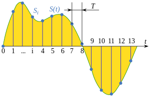 Signal sampling representation. The continuous signal
S
(
t
) is represented with a green colored line while the discrete samples are indicated by the blue vertical lines.
Signal sampling representation. The continuous signal
S
(
t
) is represented with a green colored line while the discrete samples are indicated by the blue vertical lines.
In
signal processing
,
sampling
is the reduction of a
continuous-time signal
to a
discrete-time signal
. A common example is the conversion of a
sound wave
to a sequence of "samples".
A
sample
is a value of the
signal
at a point in time and/or space; this definition differs from
the term's usage in statistics
, which refers to a set of such values.
[A]
A
sampler
is a subsystem or operation that extracts samples from a
continuous signal
. A theoretical
ideal sampler
produces samples equivalent to the instantaneous value of the continuous signal at the desired points.
The original signal can be reconstructed from a sequence of samples, up to the
Nyquist limit
, by passing the sequence of samples through a
reconstruction filter
.
Theory
[
edit
]
Functions of space, time, or any other dimension can be sampled, and similarly in two or more dimensions.
For functions that vary with time, let
S
(
t
) be a continuous function (or "signal") to be sampled, and let sampling be performed by measuring the value of the continuous function every
T
seconds, which is called the
sampling interval
or
sampling period
.
[1]
Then the sampled function is given by the sequence:
- S
(
nT
), for integer values of
n
.
The
sampling frequency
or
sampling rate
,
f
s
, is the average number of samples obtained in one second, thus
f
s
= 1/
T
, with the unit
samples per second
, sometimes referred to as
hertz
, for example 48 kHz is 48,000
samples per second
.
Reconstructing a continuous function from samples is done by interpolation algorithms. The
Whittaker?Shannon interpolation formula
is mathematically equivalent to an ideal
low-pass filter
whose input is a sequence of
Dirac delta functions
that are modulated (multiplied) by the sample values. When the time interval between adjacent samples is a constant (
T
), the sequence of delta functions is called a
Dirac comb
. Mathematically, the modulated Dirac comb is equivalent to the product of the comb function with
s
(
t
). That mathematical abstraction is sometimes referred to as
impulse sampling
.
[2]
Most sampled signals are not simply stored and reconstructed. The fidelity of a theoretical reconstruction is a common measure of the effectiveness of sampling. That fidelity is reduced when
s
(
t
) contains frequency components whose cycle length (period) is less than 2 sample intervals (see
Aliasing
). The corresponding frequency limit, in
cycles per second
(
hertz
), is 0.5 cycle/sample ×
f
s
samples/second =
f
s
/2, known as the
Nyquist frequency
of the sampler. Therefore,
s
(
t
) is usually the output of a
low-pass filter
, functionally known as an
anti-aliasing filter
. Without an anti-aliasing filter, frequencies higher than the Nyquist frequency will influence the samples in a way that is misinterpreted by the interpolation process.
[3]
Practical considerations
[
edit
]
In practice, the continuous signal is sampled using an
analog-to-digital converter
(ADC), a device with various physical limitations. This results in deviations from the theoretically perfect reconstruction, collectively referred to as
distortion
.
Various types of distortion can occur, including:
- Aliasing
. Some amount of aliasing is inevitable because only theoretical, infinitely long, functions can have no frequency content above the Nyquist frequency. Aliasing can be made
arbitrarily small
by using a
sufficiently large
order of the anti-aliasing filter.
- Aperture error
results from the fact that the sample is obtained as a time average within a sampling region, rather than just being equal to the signal value at the sampling instant.
[4]
In a
capacitor
-based
sample and hold
circuit, aperture errors are introduced by multiple mechanisms. For example, the capacitor cannot instantly track the input signal and the capacitor can not instantly be isolated from the input signal.
- Jitter
or deviation from the precise sample timing intervals.
- Noise
, including thermal sensor noise,
analog circuit
noise, etc.
- Slew rate
limit error, caused by the inability of the ADC input value to change sufficiently rapidly.
- Quantization
as a consequence of the finite precision of words that represent the converted values.
- Error due to other
non-linear
effects of the mapping of input voltage to converted output value (in addition to the effects of quantization).
Although the use of
oversampling
can completely eliminate aperture error and aliasing by shifting them out of the passband, this technique cannot be practically used above a few GHz, and may be prohibitively expensive at much lower frequencies. Furthermore, while oversampling can reduce quantization error and non-linearity, it cannot eliminate these entirely. Consequently, practical ADCs at audio frequencies typically do not exhibit aliasing, aperture error, and are not limited by quantization error. Instead, analog noise dominates. At RF and microwave frequencies where oversampling is impractical and filters are expensive, aperture error, quantization error and aliasing can be significant limitations.
Jitter, noise, and quantization are often analyzed by modeling them as random errors added to the sample values. Integration and zero-order hold effects can be analyzed as a form of
low-pass filtering
. The non-linearities of either ADC or DAC are analyzed by replacing the ideal
linear function
mapping with a proposed
nonlinear function
.
Applications
[
edit
]
Audio sampling
[
edit
]
Digital audio
uses
pulse-code modulation
(PCM) and digital signals for sound reproduction. This includes analog-to-digital conversion (ADC), digital-to-analog conversion (DAC), storage, and transmission. In effect, the system commonly referred to as digital is in fact a discrete-time, discrete-level analog of a previous electrical analog. While modern systems can be quite subtle in their methods, the primary usefulness of a digital system is the ability to store, retrieve and transmit signals without any loss of quality.
When it is necessary to capture audio covering the entire 20?20,000 Hz range of
human hearing
[5]
such as when recording music or many types of acoustic events, audio waveforms are typically sampled at 44.1 kHz (
CD
), 48 kHz, 88.2 kHz, or 96 kHz.
[6]
The approximately double-rate requirement is a consequence of the
Nyquist theorem
. Sampling rates higher than about 50 kHz to 60 kHz cannot supply more usable information for human listeners. Early
professional audio
equipment manufacturers chose sampling rates in the region of 40 to 50 kHz for this reason.
There has been an industry trend towards sampling rates well beyond the basic requirements: such as 96 kHz and even 192 kHz
[7]
Even though
ultrasonic
frequencies are inaudible to humans, recording and mixing at higher sampling rates is effective in eliminating the distortion that can be caused by
foldback aliasing
. Conversely, ultrasonic sounds may interact with and modulate the audible part of the frequency spectrum (
intermodulation distortion
),
degrading
the fidelity.
[8]
One advantage of higher sampling rates is that they can relax the low-pass filter design requirements for
ADCs
and
DACs
, but with modern oversampling
delta-sigma-converters
this advantage is less important.
The
Audio Engineering Society
recommends 48 kHz sampling rate for most applications but gives recognition to 44.1 kHz for CD and other consumer uses, 32 kHz for transmission-related applications, and 96 kHz for higher bandwidth or relaxed
anti-aliasing filtering
.
[9]
Both Lavry Engineering and J. Robert Stuart state that the ideal sampling rate would be about 60 kHz, but since this is not a standard frequency, recommend 88.2 or 96 kHz for recording purposes.
[10]
[11]
[12]
[13]
A more complete list of common audio sample rates is:
| Sampling rate
|
Use
|
| 8,000 Hz
|
Telephone
and encrypted
walkie-talkie
,
wireless intercom
and
wireless microphone
transmission; adequate for human speech but without
sibilance
(
ess
sounds like
eff
(
/
s
/
,
/
f
/
)).
|
| 11,025 Hz
|
One quarter the sampling rate of audio CDs; used for lower-quality PCM, MPEG audio and for audio analysis of subwoofer bandpasses.
[
citation needed
]
|
| 16,000 Hz
|
Wideband
frequency extension over standard
telephone
narrowband
8,000 Hz. Used in most modern
VoIP
and
VVoIP
communication products.
[14]
[
unreliable source?
]
|
| 22,050 Hz
|
One half the sampling rate of audio CDs; used for lower-quality PCM and MPEG audio and for audio analysis of low frequency energy. Suitable for digitizing early 20th century audio formats such as
78s
and
AM Radio
.
[15]
|
| 32,000 Hz
|
miniDV
digital video
camcorder
, video tapes with extra channels of audio (e.g.
DVCAM
with four channels of audio),
DAT
(LP mode), Germany's
Digitales Satellitenradio
,
NICAM
digital audio, used alongside analogue television sound in some countries. High-quality digital
wireless microphones
.
[16]
Suitable for digitizing
FM radio
.
[
citation needed
]
|
| 37,800 Hz
|
CD-XA audio
|
| 44,056 Hz
|
Used by digital audio locked to
NTSC
color
video signals (3 samples per line, 245 lines per field, 59.94 fields per second = 29.97
frames per second
).
|
| 44,100 Hz
|
Audio CD
, also most commonly used with
MPEG-1
audio (
VCD
,
SVCD
,
MP3
). Originally chosen by
Sony
because it could be recorded on modified video equipment running at either 25 frames per second (PAL) or 30 frame/s (using an NTSC
monochrome
video recorder) and cover the 20 kHz bandwidth thought necessary to match professional analog recording equipment of the time. A
PCM adaptor
would fit digital audio samples into the analog video channel of, for example,
PAL
video tapes using 3 samples per line, 588 lines per frame, 25 frames per second.
|
| 47,250 Hz
|
world's first commercial
PCM
sound recorder by
Nippon Columbia
(Denon)
|
| 48,000 Hz
|
The standard audio sampling rate used by professional digital video equipment such as tape recorders, video servers, vision mixers and so on. This rate was chosen because it could reconstruct frequencies up to 22 kHz and work with 29.97 frames per second NTSC video ? as well as 25 frame/s, 30 frame/s and 24 frame/s systems. With 29.97 frame/s systems it is necessary to handle 1601.6 audio samples per frame delivering an integer number of audio samples only every fifth video frame.
[9]
Also used for sound with consumer video formats like DV,
digital TV
,
DVD
, and films. The professional
serial digital interface
(SDI) and High-definition Serial Digital Interface (HD-SDI) used to connect broadcast television equipment together uses this audio sampling frequency. Most professional audio gear uses 48 kHz sampling, including
mixing consoles
, and
digital recording
devices.
|
| 50,000 Hz
|
First commercial digital audio recorders from the late 70s from
3M
and
Soundstream
.
|
| 50,400 Hz
|
Sampling rate used by the
Mitsubishi X-80
digital audio recorder.
|
| 64,000 Hz
|
Uncommonly used, but supported by some hardware
[17]
[18]
and software.
[19]
[20]
|
| 88,200 Hz
|
Sampling rate used by some professional recording equipment when the destination is CD (multiples of 44,100 Hz). Some pro audio gear uses (or is able to select) 88.2 kHz sampling, including mixers, EQs, compressors, reverb, crossovers and recording devices.
|
| 96,000 Hz
|
DVD-Audio
, some
LPCM
DVD tracks,
BD-ROM
(Blu-ray Disc) audio tracks,
HD DVD
(High-Definition DVD) audio tracks. Some professional recording and production equipment is able to select 96 kHz sampling. This sampling frequency is twice the 48 kHz standard commonly used with audio on professional equipment.
|
| 176,400 Hz
|
Sampling rate used by
HDCD
recorders and other professional applications for CD production. Four times the frequency of 44.1 kHz.
|
| 192,000 Hz
|
DVD-Audio
, some
LPCM
DVD tracks,
BD-ROM
(Blu-ray Disc) audio tracks, and
HD DVD
(High-Definition DVD) audio tracks, High-Definition audio recording devices and audio editing software. This sampling frequency is four times the 48 kHz standard commonly used with audio on professional video equipment.
|
| 352,800 Hz
|
Digital eXtreme Definition
, used for recording and editing
Super Audio CDs
, as 1-bit
Direct Stream Digital (DSD)
is not suited for editing. Eight times the frequency of 44.1 kHz.
|
| 2,822,400 Hz
|
SACD
, 1-bit
delta-sigma modulation
process known as
Direct Stream Digital
, co-developed by
Sony
and
Philips
.
|
| 5,644,800 Hz
|
Double-Rate DSD, 1-bit
Direct Stream Digital
at 2× the rate of the SACD. Used in some professional DSD recorders.
|
| 11,289,600 Hz
|
Quad-Rate DSD, 1-bit
Direct Stream Digital
at 4× the rate of the SACD. Used in some uncommon professional DSD recorders.
|
| 22,579,200 Hz
|
Octuple-Rate DSD, 1-bit
Direct Stream Digital
at 8× the rate of the SACD. Used in rare experimental DSD recorders. Also known as DSD512.
|
| 45,158,400 Hz
|
Sexdecuple-Rate DSD, 1-bit
Direct Stream Digital
at 16× the rate of the SACD. Used in rare experimental DSD recorders. Also known as DSD1024.
[B]
|
Bit depth
[
edit
]
Audio is typically recorded at 8-, 16-, and 24-bit depth, which yield a theoretical maximum
signal-to-quantization-noise ratio
(SQNR) for a pure
sine wave
of, approximately, 49.93
dB
, 98.09 dB and 122.17 dB.
[21]
CD quality audio uses 16-bit samples.
Thermal noise
limits the true number of bits that can be used in quantization. Few analog systems have
signal to noise ratios (SNR)
exceeding 120 dB. However,
digital signal processing
operations can have very high dynamic range, consequently it is common to perform mixing and mastering operations at 32-bit precision and then convert to 16- or 24-bit for distribution.
Speech sampling
[
edit
]
Speech signals, i.e., signals intended to carry only human
speech
, can usually be sampled at a much lower rate. For most
phonemes
, almost all of the energy is contained in the 100 Hz ? 4 kHz range, allowing a sampling rate of 8 kHz. This is the
sampling rate
used by nearly all
telephony
systems, which use the
G.711
sampling and quantization specifications.
[
citation needed
]
Video sampling
[
edit
]
Standard-definition television
(SDTV) uses either 720 by 480
pixels
(US
NTSC
525-line) or 720 by 576
pixels
(UK
PAL
625-line) for the visible picture area.
High-definition television
(HDTV) uses
720p
(progressive),
1080i
(interlaced), and
1080p
(progressive, also known as Full-HD).
In
digital video
, the temporal sampling rate is defined as the
frame rate
– or rather the
field rate
– rather than the notional
pixel clock
. The image sampling frequency is the repetition rate of the sensor integration period. Since the integration period may be significantly shorter than the time between repetitions, the sampling frequency can be different from the inverse of the sample time:
- 50 Hz ?
PAL
video
- 60 / 1.001 Hz ~= 59.94 Hz ?
NTSC
video
Video
digital-to-analog converters
operate in the megahertz range (from ~3 MHz for low quality composite video scalers in early games consoles, to 250 MHz or more for the highest-resolution VGA output).
When analog video is converted to
digital video
, a different sampling process occurs, this time at the pixel frequency, corresponding to a spatial sampling rate along
scan lines
. A common
pixel
sampling rate is:
Spatial sampling in the other direction is determined by the spacing of scan lines in the
raster
. The sampling rates and resolutions in both spatial directions can be measured in units of lines per picture height.
Spatial
aliasing
of high-frequency
luma
or
chroma
video components shows up as a
moire pattern
.
3D sampling
[
edit
]
The process of
volume rendering
samples a 3D grid of
voxels
to produce 3D renderings of sliced (tomographic) data. The 3D grid is assumed to represent a continuous region of 3D space. Volume rendering is common in medical imaging,
X-ray computed tomography
(CT/CAT),
magnetic resonance imaging
(MRI),
positron emission tomography
(PET) are some examples. It is also used for
seismic tomography
and other applications.
 The top two graphs depict Fourier transforms of two different functions that produce the same results when sampled at a particular rate. The baseband function is sampled faster than its Nyquist rate, and the bandpass function is undersampled, effectively converting it to baseband. The lower graphs indicate how identical spectral results are created by the aliases of the sampling process.
Undersampling
[
edit
]
When a
bandpass
signal is sampled slower than its
Nyquist rate
, the samples are indistinguishable from samples of a low-frequency
alias
of the high-frequency signal. That is often done purposefully in such a way that the lowest-frequency alias satisfies the
Nyquist criterion
, because the bandpass signal is still uniquely represented and recoverable. Such
undersampling
is also known as
bandpass sampling
,
harmonic sampling
,
IF sampling
, and
direct IF to digital conversion.
[22]
Oversampling
[
edit
]
Oversampling is used in most modern analog-to-digital converters to reduce the distortion introduced by practical
digital-to-analog converters
, such as a
zero-order hold
instead of idealizations like the
Whittaker?Shannon interpolation formula
.
[23]
Complex sampling
[
edit
]
Complex sampling
(or
I/Q sampling
) is the simultaneous sampling of two different, but related, waveforms, resulting in pairs of samples that are subsequently treated as
complex numbers
.
[C]
When one waveform
 is the
Hilbert transform
of the other waveform
is the
Hilbert transform
of the other waveform
 the complex-valued function,
 is called an
analytic signal
, whose Fourier transform is zero for all negative values of frequency. In that case, the
Nyquist rate
for a waveform with no frequencies ≥
B
can be reduced to just
B
(complex samples/sec), instead of 2
B
(real samples/sec).
[D]
More apparently, the
equivalent baseband waveform
,
is called an
analytic signal
, whose Fourier transform is zero for all negative values of frequency. In that case, the
Nyquist rate
for a waveform with no frequencies ≥
B
can be reduced to just
B
(complex samples/sec), instead of 2
B
(real samples/sec).
[D]
More apparently, the
equivalent baseband waveform
,
 also has a Nyquist rate of
B
, because all of its non-zero frequency content is shifted into the interval [-B/2, B/2).
also has a Nyquist rate of
B
, because all of its non-zero frequency content is shifted into the interval [-B/2, B/2).
Although complex-valued samples can be obtained as described above, they are also created by manipulating samples of a real-valued waveform. For instance, the equivalent baseband waveform can be created without explicitly computing
 by processing the product sequence
![{\displaystyle ,\left[s(nT)\cdot e^{-i2\pi {\frac {B}{2}}Tn}\right],}](https://wikimedia.org/api/rest_v1/media/math/render/svg/03e5c33cfaa6203b2cfffe7aae71115f17953f5e) [E]
through a digital low-pass filter whose cutoff frequency is
B
/2.
[F]
Computing only every other sample of the output sequence reduces the sample-rate commensurate with the reduced Nyquist rate. The result is half as many complex-valued samples as the original number of real samples. No information is lost, and the original s(t) waveform can be recovered, if necessary.
[E]
through a digital low-pass filter whose cutoff frequency is
B
/2.
[F]
Computing only every other sample of the output sequence reduces the sample-rate commensurate with the reduced Nyquist rate. The result is half as many complex-valued samples as the original number of real samples. No information is lost, and the original s(t) waveform can be recovered, if necessary.
See also
[
edit
]
Notes
[
edit
]
- ^
For example, "number of samples" in signal processing is roughly equivalent to "
sample size
" in statistics.
- ^
Even higher DSD sampling rates exist, but the benefits of those are likely imperceptible, and the size of those files would be humongous.
- ^
Sample-pairs are also sometimes viewed as points on a
constellation diagram
.
- ^
When the complex sample-rate is
B
, a frequency component at 0.6
B
, for instance, will have an alias at ?0.4
B
, which is unambiguous because of the constraint that the pre-sampled signal was analytic. Also see
Aliasing § Complex sinusoids
.
- ^
When
s
(
t
) is sampled at the Nyquist frequency (1/
T
= 2
B
), the product sequence simplifies to
![{\displaystyle \left[s(nT)\cdot (-i)^{n}\right].}](https://wikimedia.org/api/rest_v1/media/math/render/svg/7e0394ce8648cfa875d6274242b21368a4ded905)
- ^
The sequence of complex numbers is convolved with the impulse response of a filter with real-valued coefficients. That is equivalent to separately filtering the sequences of real parts and imaginary parts and reforming complex pairs at the outputs.
References
[
edit
]
- ^
Martin H. Weik (1996).
Communications Standard Dictionary
. Springer.
ISBN
0412083914
.
- ^
Rao, R. (2008).
Signals and Systems
. Prentice-Hall Of India Pvt. Limited.
ISBN
9788120338593
.
- ^
C. E. Shannon
, "Communication in the presence of noise",
Proc. Institute of Radio Engineers
, vol. 37, no.1, pp. 10?21, Jan. 1949.
Reprint as classic paper in:
Proc. IEEE
, Vol. 86, No. 2, (Feb 1998)
Archived
2010-02-08 at the
Wayback Machine
- ^
H.O. Johansson and C. Svensson, "Time resolution of NMOS sampling switches", IEEE J. Solid-State Circuits Volume: 33, Issue: 2, pp. 237?245, Feb 1998.
- ^
D'Ambrose, Christoper; Choudhary, Rizwan (2003). Elert, Glenn (ed.).
"Frequency range of human hearing"
.
The Physics Factbook
. Retrieved
2022-01-22
.
- ^
Self, Douglas (2012).
Audio Engineering Explained
. Taylor & Francis US. pp. 200, 446.
ISBN
978-0240812731
.
- ^
"Digital Pro Sound"
. Retrieved
8 January
2014
.
- ^
Colletti, Justin (February 4, 2013).
"The Science of Sample Rates (When Higher Is Better?And When It Isn't)"
.
Trust Me I'm a Scientist
. Retrieved
February 6,
2013
.
in many cases, we can hear the sound of higher sample rates not because they are more transparent, but because they are less so. They can actually introduce unintended distortion in the audible spectrum
- ^
a
b
AES5-2008: AES recommended practice for professional digital audio ? Preferred sampling frequencies for applications employing pulse-code modulation
, Audio Engineering Society, 2008
, retrieved
2010-01-18
- ^
Lavry, Dan (May 3, 2012).
"The Optimal Sample Rate for Quality Audio"
(PDF)
.
Lavry Engineering Inc
.
Although 60 KHz would be closer to the ideal; given the existing standards, 88.2 KHz and 96 KHz are closest to the optimal sample rate.
- ^
Lavry, Dan.
"The Optimal Sample Rate for Quality Audio"
.
Gearslutz
. Retrieved
2018-11-10
.
I am trying to accommodate all ears, and there are reports of few people that can actually hear slightly above 20KHz. I do think that 48KHz is pretty good compromise, but 88.2 or 96KHz yields some additional margin.
- ^
Lavry, Dan.
"To mix at 96k or not?"
.
Gearslutz
. Retrieved
2018-11-10
.
Nowdays there are a number of good designers and ear people that find 60-70KHz sample rate to be the optimal rate for the ear. It is fast enough to include what we can hear, yet slow enough to do it pretty accurately.
- ^
Stuart, J. Robert (1998).
Coding High Quality Digital Audio
.
CiteSeerX
10.1.1.501.6731
.
both psychoacoustic analysis and experience tell us that the minimum rectangular channel necessary to ensure transparency uses linear PCM with 18.2-bit samples at 58kHz. ... there are strong arguments for maintaining integer relationships with existing sampling rates ? which suggests that 88.2kHz or 96kHz should be adopted.
- ^
"Cisco VoIP Phones, Networking and Accessories - VoIP Supply"
.
- ^
"The restoration procedure ? part 1"
. Restoring78s.co.uk. Archived from
the original
on 2009-09-14
. Retrieved
2011-01-18
.
For most records a sample rate of 22050 in stereo is adequate. An exception is likely to be recordings made in the second half of the century, which may need a sample rate of 44100.
- ^
"Zaxcom digital wireless transmitters"
. Zaxcom.com. Archived from
the original
on 2011-02-09
. Retrieved
2011-01-18
.
- ^
"RME: Hammerfall DSP 9632"
.
www.rme-audio.de
. Retrieved
2018-12-18
.
Supported sample frequencies: Internally 32, 44.1, 48, 64, 88.2, 96, 176.4, 192 kHz.
- ^
"SX-S30DAB | Pioneer"
.
www.pioneer-audiovisual.eu
. Retrieved
2018-12-18
.
Supported sampling rates: 44.1 kHz, 48 kHz, 64 kHz, 88.2 kHz, 96 kHz, 176.4 kHz, 192 kHz
- ^
Cristina Bachmann, Heiko Bischoff; Schutte, Benjamin.
"Customize Sample Rate Menu"
.
Steinberg WaveLab Pro
. Retrieved
2018-12-18
.
Common Sample Rates: 64 000 Hz
- ^
"M Track 2x2M Cubase Pro 9 can ?t change Sample Rate"
.
M-Audio
. Retrieved
2018-12-18
.
[Screenshot of Cubase]
- ^
"MT-001: Taking the Mystery out of the Infamous Formula, "SNR=6.02N + 1.76dB," and Why You Should Care"
(PDF)
.
- ^
Walt Kester (2003).
Mixed-signal and DSP design techniques
. Newnes. p. 20.
ISBN
978-0-7506-7611-3
. Retrieved
8 January
2014
.
- ^
William Morris Hartmann (1997).
Signals, Sound, and Sensation
. Springer.
ISBN
1563962837
.
Further reading
[
edit
]
- Matt Pharr, Wenzel Jakob and Greg Humphreys,
Physically Based Rendering: From Theory to Implementation, 3rd ed.
, Morgan Kaufmann, November 2016.
ISBN
978-0128006450
. The chapter on sampling (
available online
) is nicely written with diagrams, core theory and code sample.
External links
[
edit
]