Classical approach to the many-body problem of astronomy
 The perturbing forces of the
Sun
on the
Moon
at two places in its
orbit
. The blue arrows represent the
direction and magnitude
of the gravitational force on the
Earth
. Applying this to both the Earth's and the Moon's position does not disturb the positions relative to each other. When it is subtracted from the force on the Moon (black arrows), what is left is the perturbing force (red arrows) on the Moon relative to the Earth. Because the perturbing force is different in direction and magnitude on opposite sides of the orbit, it produces a change in the shape of the orbit.
The perturbing forces of the
Sun
on the
Moon
at two places in its
orbit
. The blue arrows represent the
direction and magnitude
of the gravitational force on the
Earth
. Applying this to both the Earth's and the Moon's position does not disturb the positions relative to each other. When it is subtracted from the force on the Moon (black arrows), what is left is the perturbing force (red arrows) on the Moon relative to the Earth. Because the perturbing force is different in direction and magnitude on opposite sides of the orbit, it produces a change in the shape of the orbit.
In
astronomy
,
perturbation
is the complex motion of a
massive body
subjected to forces other than the
gravitational
attraction of a single other
massive
body
.
[1]
The other forces can include a third (fourth, fifth, etc.) body,
resistance
, as from an
atmosphere
, and the off-center attraction of an
oblate
or otherwise misshapen body.
[2]
Introduction
[
edit
]
The study of perturbations began with the first attempts to predict planetary motions in the sky. In ancient times the causes were unknown.
Isaac Newton
, at the time he formulated his laws of
motion
and of
gravitation
, applied them to the first analysis of perturbations,
[2]
recognizing the complex difficulties of their calculation.
[3]
Many of the great mathematicians since then have given attention to the various problems involved; throughout the 18th and 19th centuries there was demand for accurate tables of the position of the
Moon
and
planets
for
marine navigation
.
The complex motions of gravitational perturbations can be broken down. The hypothetical motion that the body follows under the gravitational effect of one other body only is a
conic section
, and can be described in
geometrical
terms. This is called a
two-body problem
, or an unperturbed
Keplerian orbit
. The differences between that and the actual motion of the body are perturbations due to the additional gravitational effects of the remaining body or bodies. If there is only one other significant body then the perturbed motion is a
three-body problem
; if there are multiple other bodies it is an
n
-body problem
. A general analytical solution (a mathematical expression to predict the positions and motions at any future time) exists for the two-body problem; when more than two bodies are considered analytic solutions exist only for special cases. Even the two-body problem becomes insoluble if one of the bodies is irregular in shape.
[4]
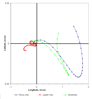 Mercury
's orbital longitude and latitude, as perturbed by
Venus
,
Jupiter
and all of the planets of the
Solar System
, at intervals of 2.5 days. Mercury would remain centered on the crosshairs if there were no perturbations.
Mercury
's orbital longitude and latitude, as perturbed by
Venus
,
Jupiter
and all of the planets of the
Solar System
, at intervals of 2.5 days. Mercury would remain centered on the crosshairs if there were no perturbations.
Most systems that involve multiple gravitational attractions present one primary body which is dominant in its effects (for example, a
star
, in the case of the star and its planet, or a planet, in the case of the planet and its satellite). The gravitational effects of the other bodies can be treated as perturbations of the hypothetical unperturbed motion of the planet or
satellite
around its primary body.
Mathematical analysis
[
edit
]
General perturbations
[
edit
]
In methods of
general perturbations
, general differential equations, either of motion or of change in the
orbital elements
, are solved analytically, usually by
series expansions
. The result is usually expressed in terms of algebraic and trigonometric functions of the orbital elements of the body in question and the perturbing bodies. This can be applied generally to many different sets of conditions, and is not specific to any particular set of gravitating objects.
[5]
Historically, general perturbations were investigated first. The classical methods are known as
variation of the elements
,
variation of parameters
or
variation of the constants of integration
. In these methods, it is considered that the body is always moving in a
conic section
, however the conic section is constantly changing due to the perturbations. If all perturbations were to cease at any particular instant, the body would continue in this (now unchanging) conic section indefinitely; this conic is known as the
osculating orbit
and its
orbital elements
at any particular time are what are sought by the methods of general perturbations.
[2]
General perturbations takes advantage of the fact that in many problems of
celestial mechanics
, the two-body orbit changes rather slowly due to the perturbations; the two-body orbit is a good first approximation. General perturbations is applicable only if the perturbing forces are about one order of magnitude smaller, or less, than the gravitational force of the primary body.
[4]
In the
Solar System
, this is usually the case;
Jupiter
, the second largest body, has a mass of about
1
⁄
1000
that of the
Sun
.
General perturbation methods are preferred for some types of problems, as the source of certain observed motions are readily found. This is not necessarily so for special perturbations; the motions would be predicted with similar accuracy, but no information on the configurations of the perturbing bodies (for instance, an
orbital resonance
) which caused them would be available.
[4]
Special perturbations
[
edit
]
In methods of
special perturbations
, numerical datasets, representing values for the positions, velocities and accelerative forces on the bodies of interest, are made the basis of
numerical integration
of the differential
equations of motion
.
[6]
In effect, the positions and velocities are perturbed directly, and no attempt is made to calculate the curves of the orbits or the
orbital elements
.
[2]
Special perturbations can be applied to any problem in
celestial mechanics
, as it is not limited to cases where the perturbing forces are small.
[4]
Once applied only to comets and minor planets, special perturbation methods are now the basis of the most accurate machine-generated
planetary ephemerides
of the great astronomical almanacs.
[2]
[7]
Special perturbations are also used for
modeling
an orbit with computers.
Cowell's formulation
[
edit
]
 Cowell's method. Forces from all perturbing bodies (black and gray) are summed to form the total force on body
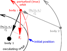
 (red), and this is numerically integrated starting from the initial position (the
epoch of osculation
).
(red), and this is numerically integrated starting from the initial position (the
epoch of osculation
).
Cowell's formulation (so named for
Philip H. Cowell
, who, with A.C.D. Cromellin, used a similar method to predict the return of Halley's comet) is perhaps the simplest of the special perturbation methods.
[8]
In a system of
 mutually interacting bodies, this method mathematically solves for the
Newtonian
forces on body
by summing the individual interactions from the other
mutually interacting bodies, this method mathematically solves for the
Newtonian
forces on body
by summing the individual interactions from the other
 bodies:

where
 is the
acceleration
vector of body
is the
acceleration
vector of body
 ,
,
 is the
gravitational constant
,
is the
gravitational constant
,
 is the
mass
of body
,
is the
mass
of body
,
 and
and
 are the
position vectors
of objects
and
are the
position vectors
of objects
and
 respectively, and
 is the distance from object
to object
, all
vectors
being referred to the
barycenter
of the system. This equation is resolved into components in
is the distance from object
to object
, all
vectors
being referred to the
barycenter
of the system. This equation is resolved into components in

 and
and
 and these are integrated numerically to form the new velocity and position vectors. This process is repeated as many times as necessary. The advantage of Cowell's method is ease of application and programming. A disadvantage is that when perturbations become large in magnitude (as when an object makes a close approach to another) the errors of the method also become large.
[9]
However, for many problems in
celestial mechanics
, this is never the case. Another disadvantage is that in systems with a dominant central body, such as the
Sun
, it is necessary to carry many
significant digits
in the
arithmetic
because of the large difference in the forces of the central body and the perturbing bodies, although with
high precision numbers
built into modern
computers
this is not as much of a limitation as it once was.
[10]
and these are integrated numerically to form the new velocity and position vectors. This process is repeated as many times as necessary. The advantage of Cowell's method is ease of application and programming. A disadvantage is that when perturbations become large in magnitude (as when an object makes a close approach to another) the errors of the method also become large.
[9]
However, for many problems in
celestial mechanics
, this is never the case. Another disadvantage is that in systems with a dominant central body, such as the
Sun
, it is necessary to carry many
significant digits
in the
arithmetic
because of the large difference in the forces of the central body and the perturbing bodies, although with
high precision numbers
built into modern
computers
this is not as much of a limitation as it once was.
[10]
Encke's method
[
edit
]
 Encke's method. Greatly exaggerated here, the small difference δ
r
(blue) between the osculating, unperturbed orbit (black) and the perturbed orbit (red), is numerically integrated starting from the initial position (the
epoch of osculation
).
Encke's method. Greatly exaggerated here, the small difference δ
r
(blue) between the osculating, unperturbed orbit (black) and the perturbed orbit (red), is numerically integrated starting from the initial position (the
epoch of osculation
).
Encke's method begins with the
osculating orbit
as a reference and integrates numerically to solve for the variation from the reference as a function of time.
[11]
Its advantages are that perturbations are generally small in magnitude, so the integration can proceed in larger steps (with resulting lesser errors), and the method is much less affected by extreme perturbations. Its disadvantage is complexity; it cannot be used indefinitely without occasionally updating the osculating orbit and continuing from there, a process known as
rectification
.
[9]
Encke's method is similar to the general perturbation method of variation of the elements, except the rectification is performed at discrete intervals rather than continuously.
[12]
Letting
 be the
radius vector
of the
osculating orbit
,
be the
radius vector
of the
osculating orbit
,
 the radius vector of the perturbed orbit, and
 the variation from the osculating orbit,
 , and the
equation of motion
of
is simply , and the
equation of motion
of
is simply
| | (
1
)
|
 . .
| | (
2
)
|
 and
and
 are just the equations of motion of
and
are just the equations of motion of
and

 for the perturbed orbit and for the perturbed orbit and
| | (
3
)
|
 for the unperturbed orbit, for the unperturbed orbit,
| | (
4
)
|
where
 is the
gravitational parameter
with
is the
gravitational parameter
with
 and
and
 the
masses
of the central body and the perturbed body,
the
masses
of the central body and the perturbed body,
 is the perturbing
acceleration
, and
is the perturbing
acceleration
, and
 and
and
 are the magnitudes of
and
.
are the magnitudes of
and
.
Substituting from equations (
3
) and (
4
) into equation (
2
),
 | | (
5
)
|
which, in theory, could be integrated twice to find
. Since the osculating orbit is easily calculated by two-body methods,
and
are accounted for and
can be solved. In practice, the quantity in the brackets,
 , is the difference of two nearly equal vectors, and further manipulation is necessary to avoid the need for extra
significant digits
.
[13]
[14]
Encke's method was more widely used before the advent of modern
computers
, when much orbit computation was performed on
mechanical calculating machines
.
, is the difference of two nearly equal vectors, and further manipulation is necessary to avoid the need for extra
significant digits
.
[13]
[14]
Encke's method was more widely used before the advent of modern
computers
, when much orbit computation was performed on
mechanical calculating machines
.
Periodic nature
[
edit
]
 Gravity Simulator
plot of the changing
orbital eccentricity
of
Mercury
,
Venus
,
Earth
, and
Mars
over the next 50,000 years. The 0 point on this plot is the year 2007.
Gravity Simulator
plot of the changing
orbital eccentricity
of
Mercury
,
Venus
,
Earth
, and
Mars
over the next 50,000 years. The 0 point on this plot is the year 2007.
In the Solar System, many of the disturbances of one planet by another are periodic, consisting of small impulses each time a planet passes another in its orbit. This causes the bodies to follow motions that are periodic or quasi-periodic – such as the Moon in its
strongly perturbed
orbit
, which is the subject of
lunar theory
. This periodic nature led to the
discovery of Neptune
in 1846 as a result of its perturbations of the orbit of
Uranus
.
On-going mutual perturbations of the planets cause long-term quasi-periodic variations in their
orbital elements
, most apparent when two planets' orbital periods are nearly in sync. For instance, five orbits of
Jupiter
(59.31 years) is nearly equal to two of
Saturn
(58.91 years). This causes large perturbations of both, with a period of 918 years, the time required for the small difference in their positions at
conjunction
to make one complete circle, first discovered by
Laplace
.
[2]
Venus
currently has the orbit with the least
eccentricity
, i.e. it is the closest to
circular
, of all the planetary orbits. In 25,000 years' time,
Earth
will have a more circular (less eccentric) orbit than Venus. It has been shown that long-term periodic disturbances within the
Solar System
can become chaotic over very long time scales; under some circumstances one or more
planets
can cross the orbit of another, leading to collisions.
[15]
The orbits of many of the minor bodies of the Solar System, such as
comets
, are often heavily perturbed, particularly by the gravitational fields of the
gas giants
. While many of these perturbations are periodic, others are not, and these in particular may represent aspects of
chaotic motion
. For example, in April 1996,
Jupiter
's gravitational influence caused the
period
of
Comet Hale?Bopp
's orbit to decrease from 4,206 to 2,380 years, a change that will not revert on any periodic basis.
[16]
See also
[
edit
]
References
[
edit
]
- Bibliography
- Footnotes
- ^
Bate, Mueller, White (1971): ch. 9, p. 385.
- ^
a
b
c
d
e
f
Moulton (1914): ch. IX
- ^
Newton in 1684 wrote: "By reason of the deviation of the Sun from the center of gravity, the centripetal force does not always tend to that immobile center, and hence the planets neither move exactly in ellipses nor revolve twice in the same orbit. Each time a planet revolves it traces a fresh orbit, as in the motion of the Moon, and each orbit depends on the combined motions of all the planets, not to mention the action of all these on each other. But to consider simultaneously all these causes of motion and to define these motions by exact laws admitting of easy calculation exceeds, if I am not mistaken, the force of any human mind." (quoted by Prof G E Smith (Tufts University), in
"Three Lectures on the Role of Theory in Science"
1. Closing the loop: Testing Newtonian Gravity, Then and Now); and Prof R F Egerton (Portland State University, Oregon) after quoting the same passage from Newton concluded:
"Here, Newton identifies the "many body problem" which remains unsolved analytically."
Archived
2005-03-10 at the
Wayback Machine
- ^
a
b
c
d
Roy (1988): ch. 6, 7.
- ^
Bate, Mueller, White (1971): p. 387; sec. 9.4.3, p. 410.
- ^
Bate, Mueller, White (1971), pp. 387?409.
- ^
See, for instance,
Jet Propulsion Laboratory Development Ephemeris
.
- ^
Cowell, P.H.; Crommelin, A.C.D. (1910). "Investigation of the Motion of Halley's Comet from 1759 to 1910".
Greenwich Observations in Astronomy
.
71
. Bellevue, for His Majesty's Stationery Office: Neill & Co.: O1.
Bibcode
:
1911GOAMM..71O...1C
.
- ^
a
b
Danby, J.M.A. (1988).
Fundamentals of Celestial Mechanics
(2nd ed.). Willmann-Bell, Inc. chapter 11.
ISBN
0-943396-20-4
.
- ^
Herget, Paul (1948).
The Computation of Orbits
. author published. p. 91 ff.
- ^
Encke, J. F. (1854).
Uber die allgemeinen Storungen der Planeten
. pp. 319?397.
- ^
Battin (1999), sec. 10.2.
- ^
Bate, Mueller, White (1971), sec. 9.3.
- ^
Roy (1988), sec. 7.4.
- ^
see references at
Stability of the Solar System
- ^
Don Yeomans (1997-04-10).
"Comet Hale?Bopp Orbit and Ephemeris Information"
. JPL/NASA
. Retrieved
2008-10-23
.
Further reading
[
edit
]
External links
[
edit
]
- Solex
(by Aldo Vitagliano) predictions for the position/orbit/close approaches of Mars
- Gravitation
Sir George Biddell Airy's 1884 book on gravitational motion and perturbations, using little or no math.(at
Google books
)