Decomposition of periodic functions into sums of simpler sinusoidal forms
A
Fourier series
(
[1]
) is an
expansion
of a
periodic function
into a sum of
trigonometric functions
. The Fourier series is an example of a
trigonometric series
, but not all trigonometric series are Fourier series.
[2]
By expressing a function as a sum of sines and cosines, many problems involving the function become easier to analyze because trigonometric functions are well understood. For example, Fourier series were first used by
Joseph Fourier
to find solutions to the
heat equation
. This application is possible because the derivatives of trigonometric functions fall into simple patterns. Fourier series cannot be used to approximate arbitrary functions, because most functions have infinitely many terms in their Fourier series, and the series do not always
converge
. Well-behaved functions, for example
smooth
functions, have Fourier series that converge to the original function. The coefficients of the Fourier series are determined by
integrals
of the function multiplied by trigonometric functions, described in
Common forms of the Fourier series
below.
The study of the
convergence of Fourier series
focus on the behaviors of the
partial sums
, which means studying the behavior of the sum as more and more terms from the series are summed. The figures below illustrate some partial Fourier series results for the components of a
square wave
.
-
A square wave (represented as the blue dot) is approximated by its sixth partial sum (represented as the purple dot), formed by summing the first six terms (represented as arrows) of the square wave's Fourier series. Each arrow starts at the vertical sum of all the arrows to its left (i.e. the previous partial sum).
-
The first four partial sums of the Fourier series for a
square wave
. As more harmonics are added, the partial sums
converge to
(become more and more like) the square wave.
-
Function

(in red) is a Fourier series sum of 6 harmonically related sine waves (in blue). Its Fourier transform

is a frequency-domain representation that reveals the amplitudes of the summed sine waves.
Fourier series are closely related to the
Fourier transform
, which can be used to find the frequency information for functions that are not periodic. Periodic functions can be identified with functions on a circle; for this reason Fourier series are the subject of
Fourier analysis
on a circle, usually denoted as
 or
or
 . The Fourier transform is also part of
Fourier analysis
, but is defined for functions on
. The Fourier transform is also part of
Fourier analysis
, but is defined for functions on
 .
.
Since Fourier's time, many different approaches to defining and understanding the concept of Fourier series have been discovered, all of which are consistent with one another, but each of which emphasizes different aspects of the topic. Some of the more powerful and elegant approaches are based on mathematical ideas and tools that were not available in Fourier's time. Fourier originally defined the Fourier series for
real
-valued functions of real arguments, and used the
sine and cosine functions
in the decomposition. Many other
Fourier-related transforms
have since been defined, extending his initial idea to many applications and birthing an
area of mathematics
called
Fourier analysis
.
Common forms of the Fourier series
[
edit
]
A Fourier series is a continuous,
periodic function
created by a summation of harmonically related sinusoidal functions. It has several different, but equivalent, forms, shown here as partial sums. But in theory
 The subscripted symbols, called
coefficients
, and the period,
The subscripted symbols, called
coefficients
, and the period,
 determine the function
 as follows
:
as follows
:
 Fig 1. The top graph shows a non-periodic function
s
(
x
) in blue defined only over the red interval from
0
to
P
. The function can be analyzed over this interval to produce the Fourier series in the bottom graph. The Fourier series is always a periodic function, even if original function
s
(
x
) isn't.
Fig 1. The top graph shows a non-periodic function
s
(
x
) in blue defined only over the red interval from
0
to
P
. The function can be analyzed over this interval to produce the Fourier series in the bottom graph. The Fourier series is always a periodic function, even if original function
s
(
x
) isn't.
Fourier series, amplitude-phase form

| | (
Eq.1
)
|
Fourier series, sine-cosine form

| | (
Eq.2
)
|
Fourier series, exponential form

| | (
Eq.3
)
|
The harmonics are indexed by an integer,
 which is also the number of cycles the corresponding sinusoids make in interval
 . Therefore, the sinusoids have
:
. Therefore, the sinusoids have
:
- a
wavelength
equal to
 in the same units as
 .
.
- a
frequency
equal to
 in the reciprocal units of
.
in the reciprocal units of
.
Clearly these series can represent functions that are just a sum of one or more of the harmonic frequencies. The remarkable thing is that it can also represent the intermediate frequencies and/or non-sinusoidal functions because of the infinite number of terms. The amplitude-phase form is particularly useful for its insight into the rationale for the series coefficients. (see
§ Derivation
) The exponential form is most easily generalized for complex-valued functions. (see
§ Complex-valued functions
)
The equivalence of these forms requires certain relationships among the coefficients. For instance, the trigonometric identity
:
Equivalence of
polar
and
rectangular
forms

| | (
Eq.4
)
|
means that
:
|

| | (
Eq.4.1
)
|
Therefore
 and
and
 are the
rectangular coordinates
of a vector with
polar coordinates
are the
rectangular coordinates
of a vector with
polar coordinates
 and
and

The coefficients can be given/assumed, such as a music synthesizer or time samples of a waveform. In the latter case, the exponential form of Fourier series synthesizes a
discrete-time Fourier transform
where variable
represents frequency instead of time.
But typically the coefficients are determined by frequency/harmonic
analysis
of a given real-valued function
 and
represents time
:
and
represents time
:
Fourier series analysis

| | (
Eq.5
)
|
The objective is for
 to converge to
 at most or all values of
in an interval of length
at most or all values of
in an interval of length
 For the
well-behaved
functions typical of physical processes, equality is customarily assumed, and the
Dirichlet conditions
provide sufficient conditions.
For the
well-behaved
functions typical of physical processes, equality is customarily assumed, and the
Dirichlet conditions
provide sufficient conditions.
The notation
 represents integration over the chosen interval. Typical choices are
![{\displaystyle [-P/2,P/2]}](https://wikimedia.org/api/rest_v1/media/math/render/svg/773e3d42ef176524eeb449749ec2bc0a83b5566a) and
and
![{\displaystyle [0,P]}](https://wikimedia.org/api/rest_v1/media/math/render/svg/e22a95e69fea5905acab328644408c110eedea0e) .
Some authors define
.
Some authors define
 because it simplifies the arguments of the sinusoid functions, at the expense of generality. And some authors assume that
is also
-periodic, in which case
approximates the entire function. The
because it simplifies the arguments of the sinusoid functions, at the expense of generality. And some authors assume that
is also
-periodic, in which case
approximates the entire function. The
 scaling factor is explained by taking a simple case
:
scaling factor is explained by taking a simple case
:
 Only the
 term of
Eq.2
is needed for convergence, with
term of
Eq.2
is needed for convergence, with
 and
and
 Accordingly
Eq.5
provides
:
Accordingly
Eq.5
provides
:
 as required.
Exponential form coefficients
[
edit
]
Another applicable identity is
Euler's formula
:
![{\displaystyle {\begin{aligned}\cos \left(2\pi {\tfrac {n}{P}}x-\varphi _{n}\right)&{}\equiv {\tfrac {1}{2}}e^{i\left(2\pi {\tfrac {n}{P}}x-\varphi _{n}\right)}+{\tfrac {1}{2}}e^{-i\left(2\pi {\tfrac {n}{P}}x-\varphi _{n}\right)}\\[6pt]&=\left({\tfrac {1}{2}}e^{-i\varphi _{n}}\right)\cdot e^{i2\pi {\tfrac {+n}{P}}x}+\left({\tfrac {1}{2}}e^{-i\varphi _{n}}\right)^{*}\cdot e^{i2\pi {\tfrac {-n}{P}}x}\end{aligned}}}](https://wikimedia.org/api/rest_v1/media/math/render/svg/2b4e16273af487d058c192627d139fe8fca55e67)
(Note
:
the ? denotes
complex conjugation
.)
Substituting this into
Eq.1
and comparison with
Eq.3
ultimately reveals
:
Exponential form coefficients
|

| | (
Eq.6
)
|
Conversely
:
Inverse relationships

Substituting
Eq.5
into
Eq.6
also reveals
:
[3]
Fourier series analysis
|
 (
all integers
) (
all integers
)
| | (
Eq.7
)
|
Complex-valued functions
[
edit
]
Eq.7
and
Eq.3
also apply when
is a complex-valued function.
[A]
This follows by expressing
 and
and
 as separate real-valued Fourier series, and

Derivation
[
edit
]
The coefficients
and
 can be understood and derived in terms of the
cross-correlation
between
and a sinusoid at frequency
. For a general frequency
can be understood and derived in terms of the
cross-correlation
between
and a sinusoid at frequency
. For a general frequency
 and an analysis interval
![{\displaystyle [x_{0},x_{0}+P],}](https://wikimedia.org/api/rest_v1/media/math/render/svg/74358f52e616039efc9b1fcc9568f99f6ae93463) the
cross-correlation function
:
the
cross-correlation function
:
 Fig 2. The blue curve is the cross-correlation of a square wave and a cosine function, as the phase lag of the cosine varies over one cycle. The amplitude and phase lag at the maximum value are the polar coordinates of one harmonic in the Fourier series expansion of the square wave. The corresponding rectangular coordinates can be determined by evaluating the cross-correlation at just two phase lags separated by 90º.
Derivation of Eq.1
![{\displaystyle \mathrm {X} _{f}(\tau )={\tfrac {2}{P}}\int _{x_{0}}^{x_{0}+P}s(x)\cdot \cos \left(2\pi f(x-\tau )\right)\,dx;\quad \tau \in \left[0,{\tfrac {1}{f}}\right]}](https://wikimedia.org/api/rest_v1/media/math/render/svg/0ae1bbd189d0cd0cdc4218a2b78ced49bcc11d89)
| | (
Eq.8
)
|
is essentially a
matched filter
, with
template
 .
The
maximum
of
.
The
maximum
of
 is a measure of the amplitude
 of frequency
 in the function
, and the value of
in the function
, and the value of
 at the maximum determines the phase
 of that frequency. Figure 2 is an example, where
is a square wave (not shown), and frequency
is the
of that frequency. Figure 2 is an example, where
is a square wave (not shown), and frequency
is the
 harmonic. It is also an example of deriving the maximum from just two samples, instead of searching the entire function. Combining
Eq.8
with
Eq.4
gives
:
harmonic. It is also an example of deriving the maximum from just two samples, instead of searching the entire function. Combining
Eq.8
with
Eq.4
gives
:
![{\displaystyle {\begin{aligned}\mathrm {X} _{n}(\varphi )&={\tfrac {2}{P}}\int _{P}s(x)\cdot \cos \left(2\pi {\tfrac {n}{P}}x-\varphi \right)\,dx;\quad \varphi \in [0,2\pi ]\\&=\cos(\varphi )\cdot \underbrace {{\tfrac {2}{P}}\int _{P}s(x)\cdot \cos \left(2\pi {\tfrac {n}{P}}x\right)\,dx} _{A}+\sin(\varphi )\cdot \underbrace {{\tfrac {2}{P}}\int _{P}s(x)\cdot \sin \left(2\pi {\tfrac {n}{P}}x\right)\,dx} _{B}\\&=\cos(\varphi )\cdot A+\sin(\varphi )\cdot B\end{aligned}}}](https://wikimedia.org/api/rest_v1/media/math/render/svg/24287ecc41a76aacf2f640f52674dbcfcee07d21)
The derivative of
 is zero at the phase of maximum correlation.

Therefore, computing
and
according to
Eq.5
creates the component's phase
of maximum correlation. And the component's amplitude is
:

Other common notations
[
edit
]
The notation
 is inadequate for discussing the Fourier coefficients of several different functions. Therefore, it is customarily replaced by a modified form of the function
(
is inadequate for discussing the Fourier coefficients of several different functions. Therefore, it is customarily replaced by a modified form of the function
(
 in this case),
such as
in this case),
such as
 or
or
![{\displaystyle S[n]}](https://wikimedia.org/api/rest_v1/media/math/render/svg/0b4222b53917b43f530116997b71049100c95586) , and functional notation often replaces subscripting
:
, and functional notation often replaces subscripting
:
![{\displaystyle {\begin{aligned}s(x)&=\sum _{n=-\infty }^{\infty }{\widehat {s}}(n)\cdot e^{i2\pi {\tfrac {n}{P}}x}&&\scriptstyle {\text{common mathematics notation}}\\&=\sum _{n=-\infty }^{\infty }S[n]\cdot e^{i2\pi {\tfrac {n}{P}}x}&&\scriptstyle {\text{common engineering notation}}\end{aligned}}}](https://wikimedia.org/api/rest_v1/media/math/render/svg/ab1656144664ad56f8ed36ac280fbf9401ea7da9)
In engineering, particularly when the variable
represents time, the coefficient sequence is called a
frequency domain
representation. Square brackets are often used to emphasize that the domain of this function is a discrete set of frequencies.
Another commonly used frequency domain representation uses the Fourier series coefficients to
modulate
a
Dirac comb
:
![{\displaystyle S(f)\ \triangleq \ \sum _{n=-\infty }^{\infty }S[n]\cdot \delta \left(f-{\frac {n}{P}}\right),}](https://wikimedia.org/api/rest_v1/media/math/render/svg/e6a4127cd2d8d239076aad35e6b82248554b6036)
where
represents a continuous frequency domain. When variable
has units of seconds,
has units of
hertz
. The "teeth" of the comb are spaced at multiples (i.e.
harmonics
) of
 , which is called the
fundamental frequency
.
, which is called the
fundamental frequency
.
 can be recovered from this representation by an
inverse Fourier transform
:
can be recovered from this representation by an
inverse Fourier transform
:
![{\displaystyle {\begin{aligned}{\mathcal {F}}^{-1}\{S(f)\}&=\int _{-\infty }^{\infty }\left(\sum _{n=-\infty }^{\infty }S[n]\cdot \delta \left(f-{\frac {n}{P}}\right)\right)e^{i2\pi fx}\,df,\\[6pt]&=\sum _{n=-\infty }^{\infty }S[n]\cdot \int _{-\infty }^{\infty }\delta \left(f-{\frac {n}{P}}\right)e^{i2\pi fx}\,df,\\[6pt]&=\sum _{n=-\infty }^{\infty }S[n]\cdot e^{i2\pi {\tfrac {n}{P}}x}\ \ \triangleq \ s_{\infty }(x).\end{aligned}}}](https://wikimedia.org/api/rest_v1/media/math/render/svg/10002996a7c3e5b28df028d7096c4c00efee99c6)
The constructed function
is therefore commonly referred to as a
Fourier transform
, even though the Fourier integral of a periodic function is not convergent at the harmonic frequencies.
[B]
Analysis example
[
edit
]
 Plot of the
sawtooth wave
, a periodic continuation of the linear function
Plot of the
sawtooth wave
, a periodic continuation of the linear function
 on the interval
![{\displaystyle (-\pi ,\pi ]}](https://wikimedia.org/api/rest_v1/media/math/render/svg/7fbb1843079a9df3d3bbcce3249bb2599790de9c)
 Animated plot of the first five successive partial Fourier series
Consider a sawtooth function
:


In this case, the Fourier coefficients are given by
![{\displaystyle {\begin{aligned}A_{n}&={\frac {1}{\pi }}\int _{-\pi }^{\pi }s(x)\cos(nx)\,dx=0,\quad n\geq 0.\\[4pt]B_{n}&={\frac {1}{\pi }}\int _{-\pi }^{\pi }s(x)\sin(nx)\,dx\\[4pt]&=-{\frac {2}{\pi n}}\cos(n\pi )+{\frac {2}{\pi ^{2}n^{2}}}\sin(n\pi )\\[4pt]&={\frac {2\,(-1)^{n+1}}{\pi n}},\quad n\geq 1.\end{aligned}}}](https://wikimedia.org/api/rest_v1/media/math/render/svg/60820ad01df637675beb2c56a9db388cd0539490)
It can be shown that the Fourier series converges to
at every point
where
 is differentiable, and therefore
:
is differentiable, and therefore
:
![{\displaystyle {\begin{aligned}s(x)&={\frac {a_{0}}{2}}+\sum _{n=1}^{\infty }\left[A_{n}\cos \left(nx\right)+B_{n}\sin \left(nx\right)\right]\\[4pt]&={\frac {2}{\pi }}\sum _{n=1}^{\infty }{\frac {(-1)^{n+1}}{n}}\sin(nx),\quad \mathrm {for} \ (x-\pi )\ {\text{is not a multiple of}}\ 2\pi .\end{aligned}}}](https://wikimedia.org/api/rest_v1/media/math/render/svg/4b5b85f18c97953fdf678240a1f7d70bc15abbdb)
| | (
Eq.9
)
|
When
 , the Fourier series converges to 0, which is the half-sum of the left- and right-limit of
s
at
. This is a particular instance of the
Dirichlet theorem
for Fourier series.
, the Fourier series converges to 0, which is the half-sum of the left- and right-limit of
s
at
. This is a particular instance of the
Dirichlet theorem
for Fourier series.
This example leads to a solution of the
Basel problem
.
Convergence
[
edit
]
A proof that a Fourier series is a valid representation of any periodic function (that satisfies the
Dirichlet conditions
) is overviewed in
§ Fourier theorem proving convergence of Fourier series
.
In
engineering
applications, the Fourier series is generally assumed to converge except at jump discontinuities since the functions encountered in engineering are better-behaved than functions encountered in other disciplines. In particular, if
is continuous and the derivative of
(which may not exist everywhere) is square integrable, then the Fourier series of
converges absolutely and uniformly to
.
[4]
If a function is
square-integrable
on the interval
![{\displaystyle [x_{0},x_{0}+P]}](https://wikimedia.org/api/rest_v1/media/math/render/svg/3ef79a1b836ec65eacb0d2c73464996d2b7830ba) , then the Fourier series
converges
to the function at
almost everywhere
. It is possible to define Fourier coefficients for more general functions or distributions, in which case point wise convergence often fails, and convergence in norm or
weak convergence
is usually studied.
, then the Fourier series
converges
to the function at
almost everywhere
. It is possible to define Fourier coefficients for more general functions or distributions, in which case point wise convergence often fails, and convergence in norm or
weak convergence
is usually studied.
-
Four partial sums (Fourier series) of lengths 1, 2, 3, and 4 terms, showing how the approximation to a square wave improves as the number of terms increases
(animation)
-
Four partial sums (Fourier series) of lengths 1, 2, 3, and 4 terms, showing how the approximation to a sawtooth wave improves as the number of terms increases
(animation)
-
Example of convergence to a somewhat arbitrary function. Note the development of the "ringing" (
Gibbs phenomenon
) at the transitions to/from the vertical sections.
History
[
edit
]
The Fourier series is named in honor of
Jean-Baptiste Joseph Fourier
(1768?1830), who made important contributions to the study of
trigonometric series
, after preliminary investigations by
Leonhard Euler
,
Jean le Rond d'Alembert
, and
Daniel Bernoulli
.
[C]
Fourier introduced the series for the purpose of solving the
heat equation
in a metal plate, publishing his initial results in his 1807
Memoire sur la propagation de la chaleur dans les corps solides
(
Treatise on the propagation of heat in solid bodies
), and publishing his
Theorie analytique de la chaleur
(
Analytical theory of heat
) in 1822. The
Memoire
introduced Fourier analysis, specifically Fourier series. Through Fourier's research the fact was established that an arbitrary (at first, continuous
[5]
and later generalized to any
piecewise
-smooth
[6]
) function can be represented by a trigonometric series. The first announcement of this great discovery was made by Fourier in 1807, before the
French Academy
.
[7]
Early ideas of decomposing a periodic function into the sum of simple oscillating functions date back to the 3rd century BC, when ancient astronomers proposed an empiric model of planetary motions, based on
deferents and epicycles
.
The
heat equation
is a
partial differential equation
. Prior to Fourier's work, no solution to the heat equation was known in the general case, although particular solutions were known if the heat source behaved in a simple way, in particular, if the heat source was a
sine
or
cosine
wave. These simple solutions are now sometimes called
eigensolutions
. Fourier's idea was to model a complicated heat source as a superposition (or
linear combination
) of simple sine and cosine waves, and to write the
solution as a superposition
of the corresponding
eigensolutions
. This superposition or linear combination is called the Fourier series.
From a modern point of view, Fourier's results are somewhat informal, due to the lack of a precise notion of
function
and
integral
in the early nineteenth century. Later,
Peter Gustav Lejeune Dirichlet
[8]
and
Bernhard Riemann
[9]
[10]
[11]
expressed Fourier's results with greater precision and formality.
Although the original motivation was to solve the heat equation, it later became obvious that the same techniques could be applied to a wide array of mathematical and physical problems, and especially those involving linear differential equations with constant coefficients, for which the eigensolutions are
sinusoids
. The Fourier series has many such applications in
electrical engineering
,
vibration
analysis,
acoustics
,
optics
,
signal processing
,
image processing
,
quantum mechanics
,
econometrics
,
[12]
shell theory
,
[13]
etc.
Beginnings
[
edit
]
Joseph Fourier wrote:
[
dubious
–
discuss
]

Multiplying both sides by
 , and then integrating from
 to
to
 yields:

This immediately gives any coefficient
a
k
of the
trigonometrical series
for φ(
y
) for any function which has such an expansion. It works because if φ has such an expansion, then (under suitable convergence assumptions) the integral

can be carried out term-by-term. But all terms involving

for
j
≠
k
vanish when integrated from ?1 to 1, leaving only the

term.
In these few lines, which are close to the modern
formalism
used in Fourier series, Fourier revolutionized both mathematics and physics. Although similar trigonometric series were previously used by
Euler
,
d'Alembert
,
Daniel Bernoulli
and
Gauss
, Fourier believed that such trigonometric series could represent any arbitrary function. In what sense that is actually true is a somewhat subtle issue and the attempts over many years to clarify this idea have led to important discoveries in the theories of
convergence
,
function spaces
, and
harmonic analysis
.
When Fourier submitted a later competition essay in 1811, the committee (which included
Lagrange
,
Laplace
,
Malus
and
Legendre
, among others) concluded:
...the manner in which the author arrives at these equations is not exempt of difficulties and...his analysis to integrate them still leaves something to be desired on the score of generality and even
rigour
.
[
citation needed
]
Fourier's motivation
[
edit
]
 Heat distribution in a metal plate, using Fourier's method
The Fourier series expansion of the sawtooth function (above) looks more complicated than the simple formula
 , so it is not immediately apparent why one would need the Fourier series. While there are many applications, Fourier's motivation was in solving the
heat equation
. For example, consider a metal plate in the shape of a square whose sides measure
, so it is not immediately apparent why one would need the Fourier series. While there are many applications, Fourier's motivation was in solving the
heat equation
. For example, consider a metal plate in the shape of a square whose sides measure
 meters, with coordinates
![{\displaystyle (x,y)\in [0,\pi ]\times [0,\pi ]}](https://wikimedia.org/api/rest_v1/media/math/render/svg/c18734f151b17b5d3e325f79c7000826ab832610) . If there is no heat source within the plate, and if three of the four sides are held at 0 degrees Celsius, while the fourth side, given by
. If there is no heat source within the plate, and if three of the four sides are held at 0 degrees Celsius, while the fourth side, given by
 , is maintained at the temperature gradient
 degrees Celsius, for
in
degrees Celsius, for
in
 , then one can show that the stationary heat distribution (or the heat distribution after a long period of time has elapsed) is given by

Here, sinh is the
hyperbolic sine
function. This solution of the heat equation is obtained by multiplying each term of
Eq.9
by
 . While our example function
seems to have a needlessly complicated Fourier series, the heat distribution
. While our example function
seems to have a needlessly complicated Fourier series, the heat distribution
 is nontrivial. The function
 cannot be written as a
closed-form expression
. This method of solving the heat problem was made possible by Fourier's work.
cannot be written as a
closed-form expression
. This method of solving the heat problem was made possible by Fourier's work.
Complex Fourier series animation
[
edit
]
Complex Fourier series tracing the letter 'e'. (The
Julia
source code that generates the frames of this animation is here
[15]
in Appendix B.)
An example of the ability of the complex Fourier series to trace any two dimensional closed figure is shown in the adjacent animation of the complex Fourier series tracing the letter 'e' (for exponential). Note that the animation uses the variable 't' to parameterize the letter 'e' in the complex plane, which is equivalent to using the parameter 'x' in this article's subsection on complex valued functions.
In the animation's back plane, the rotating vectors are aggregated in an order that alternates between a vector rotating in the positive (counter clockwise) direction and a vector rotating at the same frequency but in the negative (clockwise) direction, resulting in a single tracing arm with lots of zigzags. This perspective shows how the addition of each pair of rotating vectors (one rotating in the positive direction and one rotating in the negative direction) nudges the previous trace (shown as a light gray dotted line) closer to the shape of the letter 'e'.
In the animation's front plane, the rotating vectors are aggregated into two sets, the set of all the positive rotating vectors and the set of all the negative rotating vectors (the non-rotating component is evenly split between the two), resulting in two tracing arms rotating in opposite directions. The animation's small circle denotes the midpoint between the two arms and also the midpoint between the origin and the current tracing point denoted by '+'. This perspective shows how the complex Fourier series is an extension (the addition of an arm) of the complex geometric series which has just one arm. It also shows how the two arms coordinate with each other. For example, as the tracing point is rotating in the positive direction, the negative direction arm stays parked. Similarly, when the tracing point is rotating in the negative direction, the positive direction arm stays parked.
In between the animation's back and front planes are rotating trapezoids whose areas represent the values of the complex Fourier series terms. This perspective shows the amplitude, frequency, and phase of the individual terms of the complex Fourier series in relation to the series sum spatially converging to the letter 'e' in the back and front planes. The audio track's left and right channels correspond respectively to the real and imaginary components of the current tracing point '+' but increased in frequency by a factor of 3536 so that the animation's fundamental frequency (n=1) is a 220 Hz tone (A220).
Other applications
[
edit
]
Another application is to solve the
Basel problem
by using
Parseval's theorem
. The example generalizes and one may compute
ζ
(2
n
), for any positive integer
n
.
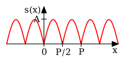
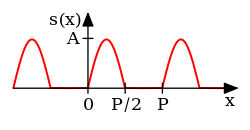
Table of common Fourier series
[
edit
]
Some common pairs of periodic functions and their Fourier series coefficients are shown in the table below.
- designates a periodic function with period
.
 designate the Fourier series coefficients (sine-cosine form) of the periodic function
.
designate the Fourier series coefficients (sine-cosine form) of the periodic function
.
Time domain
|
Plot
|
Frequency domain (sine-cosine form)

|
Remarks
|
Reference
|

|
|

|
Full-wave rectified sine
|
[16]
: p. 193
|

|
|

|
Half-wave rectified sine
|
[16]
: p. 193
|

|

|

|

|
|

|

|

|
|
[16]
: p. 192
|

|
|

|
|
[16]
: p. 192
|

|

|

|
|
[16]
: p. 193
|
Table of basic properties
[
edit
]
This table shows some mathematical operations in the time domain and the corresponding effect in the Fourier series coefficients. Notation:
- Complex conjugation
is denoted by an asterisk.
 designate
-periodic functions
or
functions defined only for
designate
-periodic functions
or
functions defined only for
![{\displaystyle x\in [0,P].}](https://wikimedia.org/api/rest_v1/media/math/render/svg/06b058e43f16179590921d9669ac45cec21a975e)
![{\displaystyle S[n],R[n]}](https://wikimedia.org/api/rest_v1/media/math/render/svg/320b593144d771f4aac1aae12d9513debbd3b20f) designate the Fourier series coefficients (exponential form) of
and
designate the Fourier series coefficients (exponential form) of
and

| Property
|
Time domain
|
Frequency domain (exponential form)
|
Remarks
|
Reference
|
| Linearity
|

|
![{\displaystyle a\cdot S[n]+b\cdot R[n]}](https://wikimedia.org/api/rest_v1/media/math/render/svg/23622be4a50d54928d05c273e803240a2cb1e413)
|

|
|
| Time reversal / Frequency reversal
|

|
![{\displaystyle S[-n]}](https://wikimedia.org/api/rest_v1/media/math/render/svg/ab628b28c49c04cab81d0bd30d19ee0797b0587c)
|
|
[17]
: p. 610
|
| Time conjugation
|

|
![{\displaystyle S^{*}[-n]}](https://wikimedia.org/api/rest_v1/media/math/render/svg/a3f6ea8a947b86f8a31046070359f6b8111a0bae)
|
|
[17]
: p. 610
|
| Time reversal & conjugation
|

|
![{\displaystyle S^{*}[n]}](https://wikimedia.org/api/rest_v1/media/math/render/svg/3776c67c40997d8044720ef84de7575679cf9638)
|
|
|
| Real part in time
|

|
![{\displaystyle {\frac {1}{2}}(S[n]+S^{*}[-n])}](https://wikimedia.org/api/rest_v1/media/math/render/svg/2eb44dffaae6c85870914249c054e33236b02cc8)
|
|
|
| Imaginary part in time
|

|
![{\displaystyle {\frac {1}{2i}}(S[n]-S^{*}[-n])}](https://wikimedia.org/api/rest_v1/media/math/render/svg/bc039a9c12ae20a4b47337ae55bf8a7bc26d2e11)
|
|
|
| Real part in frequency
|

|
![{\displaystyle \operatorname {Re} {(S[n])}}](https://wikimedia.org/api/rest_v1/media/math/render/svg/140ebff319eb8eb7965d0ca86dcaadb21685177a)
|
|
|
| Imaginary part in frequency
|

|
![{\displaystyle \operatorname {Im} {(S[n])}}](https://wikimedia.org/api/rest_v1/media/math/render/svg/0c726948120015ce0d482f5f7f4af81713342b5c)
|
|
|
| Shift in time / Modulation in frequency
|

|
![{\displaystyle S[n]\cdot e^{-i2\pi {\tfrac {x_{0}}{P}}n}}](https://wikimedia.org/api/rest_v1/media/math/render/svg/7c56731e1382c8189ca81104cbade4d310fd72d8)
|

|
[17]
: p.610
|
| Shift in frequency / Modulation in time
|

|
![{\displaystyle S[n-n_{0}]\!}](https://wikimedia.org/api/rest_v1/media/math/render/svg/07385c0e5fd45d4e07a279a91668cf8894963e0c)
|

|
[17]
: p. 610
|
Symmetry properties
[
edit
]
When the real and imaginary parts of a complex function are decomposed into their
even and odd parts
, there are four components, denoted below by the subscripts RE, RO, IE, and IO. And there is a one-to-one mapping between the four components of a complex time function and the four components of its complex frequency transform:
[18]

From this, various relationships are apparent, for example:
- The transform of a real-valued function (
s
RE
+
s
RO
) is the
even symmetric
function
S
RE
+
i
S
IO
. Conversely, an even-symmetric transform implies a real-valued time-domain.
- The transform of an imaginary-valued function (
i
s
IE
+
i
s
IO
) is the
odd symmetric
function
S
RO
+
i
S
IE
, and the converse is true.
- The transform of an even-symmetric function (
s
RE
+
i
s
IO
) is the real-valued function
S
RE
+
S
RO
, and the converse is true.
- The transform of an odd-symmetric function (
s
RO
+
i
s
IE
) is the imaginary-valued function
i
S
IE
+
i
S
IO
, and the converse is true.
Other properties
[
edit
]
Riemann?Lebesgue lemma
[
edit
]
If
 is
integrable
,
is
integrable
,
![{\textstyle \lim _{|n|\to \infty }S[n]=0}](https://wikimedia.org/api/rest_v1/media/math/render/svg/7fc04d857f6462ae29422edcada981c8a798d4b5) ,
,
 and
and
 This result is known as the
Riemann?Lebesgue lemma
.
This result is known as the
Riemann?Lebesgue lemma
.
Parseval's theorem
[
edit
]
If
belongs to
 (periodic over an interval of length
) then
:
(periodic over an interval of length
) then
:
![{\textstyle {\frac {1}{P}}\int _{P}|s(x)|^{2}\,dx=\sum _{n=-\infty }^{\infty }{\Bigl |}S[n]{\Bigr |}^{2}.}](https://wikimedia.org/api/rest_v1/media/math/render/svg/90e7f4dd99392022f87674ed1c8ea8306634bc28)
Plancherel's theorem
[
edit
]
If
 are coefficients and
 then there is a unique function
 such that
![{\displaystyle S[n]=c_{n}}](https://wikimedia.org/api/rest_v1/media/math/render/svg/c4375307afdf29e78a31ef64b699dcb3e2fde140) for every
for every
 .
.
Convolution theorems
[
edit
]
Given
-periodic functions,
 and
and
 with Fourier series coefficients
and
with Fourier series coefficients
and
![{\displaystyle R[n],}](https://wikimedia.org/api/rest_v1/media/math/render/svg/80d8bbe147f3eb3fb318d09437a3540e054b0289)

- The pointwise product
:

 sequences
:
sequences
:
![{\displaystyle H[n]=\{S*R\}[n].}](https://wikimedia.org/api/rest_v1/media/math/render/svg/b5d3978629d1c2cd954f884509a1bb360f01cac5)
- The
periodic convolution
:

![{\displaystyle H[n]=P\cdot S[n]\cdot R[n].}](https://wikimedia.org/api/rest_v1/media/math/render/svg/1804f502413d4e3e5f28f8715c52e2a3d7e7e9a6)
- A
doubly infinite
sequence
 in
in
 is the sequence of Fourier coefficients of a function in
![{\displaystyle L^{1}([0,2\pi ])}](https://wikimedia.org/api/rest_v1/media/math/render/svg/bd16426bda528c05e32e97bfba7f51b598c081b8) if and only if it is a convolution of two sequences in
if and only if it is a convolution of two sequences in
 . See
[19]
. See
[19]
Derivative property
[
edit
]
We say that
belongs to
 if
is a 2
π
-periodic function on
if
is a 2
π
-periodic function on
 which is
 times differentiable, and its
derivative is continuous.
times differentiable, and its
derivative is continuous.
- If
 , then the Fourier coefficients
![{\displaystyle {\widehat {s'}}[n]}](https://wikimedia.org/api/rest_v1/media/math/render/svg/a50845d25c79fe9547d0194fce67a390efc1a4ed) of the derivative
of the derivative
 can be expressed in terms of the Fourier coefficients
![{\displaystyle {\widehat {s}}[n]}](https://wikimedia.org/api/rest_v1/media/math/render/svg/efb5adbeb52d198894dc8f70ec8c434f0e193e6b) of the function
, via the formula
of the function
, via the formula
![{\displaystyle {\widehat {s'}}[n]=in{\widehat {s}}[n]}](https://wikimedia.org/api/rest_v1/media/math/render/svg/d281471757291b705a757faa55af0f1cebf8a0b6) .
.
- If
 , then
![{\displaystyle {\widehat {s^{(k)}}}[n]=(in)^{k}{\widehat {s}}[n]}](https://wikimedia.org/api/rest_v1/media/math/render/svg/b0120eafbcb1c02b4c2f81f5589fdc328c28bd20) . In particular, since for a fixed
. In particular, since for a fixed
 we have
![{\displaystyle {\widehat {s^{(k)}}}[n]\to 0}](https://wikimedia.org/api/rest_v1/media/math/render/svg/0ddeff4d322091a8ec85a30a10d584d426d703b1) as
as
 , it follows that
![{\displaystyle |n|^{k}{\widehat {s}}[n]}](https://wikimedia.org/api/rest_v1/media/math/render/svg/541244c281f9472e99fca9b32f2cd7676434d09c) tends to zero, which means that the Fourier coefficients converge to zero faster than the
k
th power of
n
for any
.
tends to zero, which means that the Fourier coefficients converge to zero faster than the
k
th power of
n
for any
.
Compact groups
[
edit
]
One of the interesting properties of the Fourier transform which we have mentioned, is that it carries convolutions to pointwise products. If that is the property which we seek to preserve, one can produce Fourier series on any
compact group
. Typical examples include those
classical groups
that are compact. This generalizes the Fourier transform to all spaces of the form
L
2
(
G
), where
G
is a compact group, in such a way that the Fourier transform carries
convolutions
to pointwise products. The Fourier series exists and converges in similar ways to the
[?
π
,
π
]
case.
An alternative extension to compact groups is the
Peter?Weyl theorem
, which proves results about representations of compact groups analogous to those about finite groups.
 The
atomic orbitals
of
chemistry
are partially described by
spherical harmonics
, which can be used to produce Fourier series on the
sphere
.
The
atomic orbitals
of
chemistry
are partially described by
spherical harmonics
, which can be used to produce Fourier series on the
sphere
.
Riemannian manifolds
[
edit
]
If the domain is not a group, then there is no intrinsically defined convolution. However, if
 is a
compact
Riemannian manifold
, it has a
Laplace?Beltrami operator
. The Laplace?Beltrami operator is the differential operator that corresponds to
Laplace operator
for the Riemannian manifold
. Then, by analogy, one can consider heat equations on
. Since Fourier arrived at his basis by attempting to solve the heat equation, the natural generalization is to use the eigensolutions of the Laplace?Beltrami operator as a basis. This generalizes Fourier series to spaces of the type
is a
compact
Riemannian manifold
, it has a
Laplace?Beltrami operator
. The Laplace?Beltrami operator is the differential operator that corresponds to
Laplace operator
for the Riemannian manifold
. Then, by analogy, one can consider heat equations on
. Since Fourier arrived at his basis by attempting to solve the heat equation, the natural generalization is to use the eigensolutions of the Laplace?Beltrami operator as a basis. This generalizes Fourier series to spaces of the type
 , where
is a Riemannian manifold. The Fourier series converges in ways similar to the
, where
is a Riemannian manifold. The Fourier series converges in ways similar to the
![{\displaystyle [-\pi ,\pi ]}](https://wikimedia.org/api/rest_v1/media/math/render/svg/cb064fd6c55820cfa660eabeeda0f6e3c4935ae6) case. A typical example is to take
to be the sphere with the usual metric, in which case the Fourier basis consists of
spherical harmonics
.
case. A typical example is to take
to be the sphere with the usual metric, in which case the Fourier basis consists of
spherical harmonics
.
Locally compact Abelian groups
[
edit
]
The generalization to compact groups discussed above does not generalize to noncompact,
nonabelian groups
. However, there is a straightforward generalization to
Locally Compact Abelian (LCA) groups
.
This generalizes the Fourier transform to
 or
or
 , where
 is an LCA group. If
is compact, one also obtains a Fourier series, which converges similarly to the
case, but if
is noncompact, one obtains instead a
Fourier integral
. This generalization yields the usual
Fourier transform
when the underlying locally compact Abelian group is
.
is an LCA group. If
is compact, one also obtains a Fourier series, which converges similarly to the
case, but if
is noncompact, one obtains instead a
Fourier integral
. This generalization yields the usual
Fourier transform
when the underlying locally compact Abelian group is
.
Extensions
[
edit
]
Fourier series on a square
[
edit
]
We can also define the Fourier series for functions of two variables
and
 in the square
![{\displaystyle [-\pi ,\pi ]\times [-\pi ,\pi ]}](https://wikimedia.org/api/rest_v1/media/math/render/svg/df436805f50de7386abdb2a9d058672ec1b4cebb) :
:
![{\displaystyle {\begin{aligned}f(x,y)&=\sum _{j,k\in \mathbb {Z} }c_{j,k}e^{ijx}e^{iky},\\[5pt]c_{j,k}&={\frac {1}{4\pi ^{2}}}\int _{-\pi }^{\pi }\int _{-\pi }^{\pi }f(x,y)e^{-ijx}e^{-iky}\,dx\,dy.\end{aligned}}}](https://wikimedia.org/api/rest_v1/media/math/render/svg/aec3723d7051701ab4530dce39f1480cef835981)
Aside from being useful for solving partial differential equations such as the heat equation, one notable application of Fourier series on the square is in
image compression
. In particular, the
JPEG
image compression standard uses the two-dimensional
discrete cosine transform
, a discrete form of the
Fourier cosine transform
, which uses only cosine as the basis function.
For two-dimensional arrays with a staggered appearance, half of the Fourier series coefficients disappear, due to additional symmetry.
[20]
Fourier series of Bravais-lattice-periodic-function
[
edit
]
A three-dimensional
Bravais lattice
is defined as the set of vectors of the form:

where

are integers and

are three linearly independent vectors. Assuming we have some function,

, such that it obeys the condition of periodicity for any Bravais lattice vector

,

, we could make a Fourier series of it. This kind of function can be, for example, the effective potential that one electron "feels" inside a periodic crystal. It is useful to make the Fourier series of the potential when applying
Bloch's theorem
. First, we may write any arbitrary position vector

in the coordinate-system of the lattice:

where

meaning that

is defined to be the magnitude of
, so

is the unit vector directed along
.
Thus we can define a new function,

This new function,
 , is now a function of three-variables, each of which has periodicity
 ,
,
 , and
, and
 respectively:

This enables us to build up a set of Fourier coefficients, each being indexed by three independent integers
 . In what follows, we use function notation to denote these coefficients, where previously we used subscripts. If we write a series for
 on the interval
![{\displaystyle \left[0,a_{1}\right]}](https://wikimedia.org/api/rest_v1/media/math/render/svg/187cf2c27876a96c668f73266f673002808773ac) for
for
 , we can define the following:

And then we can write:

Further defining:
![{\displaystyle {\begin{aligned}h^{\mathrm {two} }(m_{1},m_{2},x_{3})&\triangleq {\frac {1}{a_{2}}}\int _{0}^{a_{2}}h^{\mathrm {one} }(m_{1},x_{2},x_{3})\cdot e^{-i2\pi {\tfrac {m_{2}}{a_{2}}}x_{2}}\,dx_{2}\\[12pt]&={\frac {1}{a_{2}}}\int _{0}^{a_{2}}dx_{2}{\frac {1}{a_{1}}}\int _{0}^{a_{1}}dx_{1}g(x_{1},x_{2},x_{3})\cdot e^{-i2\pi \left({\tfrac {m_{1}}{a_{1}}}x_{1}+{\tfrac {m_{2}}{a_{2}}}x_{2}\right)}\end{aligned}}}](https://wikimedia.org/api/rest_v1/media/math/render/svg/257f40440f195f996a7a7df57b110f544e8553c6)
We can write
once again as:

Finally applying the same for the third coordinate, we define:
![{\displaystyle {\begin{aligned}h^{\mathrm {three} }(m_{1},m_{2},m_{3})&\triangleq {\frac {1}{a_{3}}}\int _{0}^{a_{3}}h^{\mathrm {two} }(m_{1},m_{2},x_{3})\cdot e^{-i2\pi {\tfrac {m_{3}}{a_{3}}}x_{3}}\,dx_{3}\\[12pt]&={\frac {1}{a_{3}}}\int _{0}^{a_{3}}dx_{3}{\frac {1}{a_{2}}}\int _{0}^{a_{2}}dx_{2}{\frac {1}{a_{1}}}\int _{0}^{a_{1}}dx_{1}g(x_{1},x_{2},x_{3})\cdot e^{-i2\pi \left({\tfrac {m_{1}}{a_{1}}}x_{1}+{\tfrac {m_{2}}{a_{2}}}x_{2}+{\tfrac {m_{3}}{a_{3}}}x_{3}\right)}\end{aligned}}}](https://wikimedia.org/api/rest_v1/media/math/render/svg/e16c337b17dc4ed299de47b108a2ff7eb060b9f3)
We write
as:

Re-arranging:

Now, every
reciprocal
lattice vector can be written (but does not mean that it is the only way of writing) as
 , where
 are integers and
 are reciprocal lattice vectors to satisfy
 (
(
 for
for
 , and
, and
 for
for
 ). Then for any arbitrary reciprocal lattice vector
 and arbitrary position vector
in the original Bravais lattice space, their scalar product is:
and arbitrary position vector
in the original Bravais lattice space, their scalar product is:

So it is clear that in our expansion of
 , the sum is actually over reciprocal lattice vectors:

where

Assuming

we can solve this system of three linear equations for
,
, and

in terms of
,

and

in order to calculate the volume element in the original rectangular coordinate system. Once we have
,
, and
in terms of
,
and
, we can calculate the
Jacobian determinant
:
![{\displaystyle {\begin{vmatrix}{\dfrac {\partial x_{1}}{\partial x}}&{\dfrac {\partial x_{1}}{\partial y}}&{\dfrac {\partial x_{1}}{\partial z}}\\[12pt]{\dfrac {\partial x_{2}}{\partial x}}&{\dfrac {\partial x_{2}}{\partial y}}&{\dfrac {\partial x_{2}}{\partial z}}\\[12pt]{\dfrac {\partial x_{3}}{\partial x}}&{\dfrac {\partial x_{3}}{\partial y}}&{\dfrac {\partial x_{3}}{\partial z}}\end{vmatrix}}}](https://wikimedia.org/api/rest_v1/media/math/render/svg/5e5df9134486606d6a55c8ec4a96ee3ca353e924)
which after some calculation and applying some non-trivial cross-product identities can be shown to be equal to:

(it may be advantageous for the sake of simplifying calculations, to work in such a rectangular coordinate system, in which it just so happens that
 is parallel to the
x
axis,
is parallel to the
x
axis,
 lies in the
xy
-plane, and
lies in the
xy
-plane, and
 has components of all three axes). The denominator is exactly the volume of the primitive unit cell which is enclosed by the three primitive-vectors
,
and
. In particular, we now know that
has components of all three axes). The denominator is exactly the volume of the primitive unit cell which is enclosed by the three primitive-vectors
,
and
. In particular, we now know that

We can write now
 as an integral with the traditional coordinate system over the volume of the primitive cell, instead of with the
,
and
variables:
as an integral with the traditional coordinate system over the volume of the primitive cell, instead of with the
,
and
variables:

writing

for the volume element

; and where

is the primitive unit cell, thus,

is the volume of the primitive unit cell.
Hilbert space interpretation
[
edit
]
In the language of
Hilbert spaces
, the set of functions
 is an
orthonormal basis
for the space
is an
orthonormal basis
for the space
![{\displaystyle L^{2}([-\pi ,\pi ])}](https://wikimedia.org/api/rest_v1/media/math/render/svg/0f84fea7a212acaf14649b6cdcca282b0646a8b0) of square-integrable functions on
. This space is actually a Hilbert space with an
inner product
given for any two elements
and
by:
of square-integrable functions on
. This space is actually a Hilbert space with an
inner product
given for any two elements
and
by:
 where
where
 is the complex conjugate of

The basic Fourier series result for Hilbert spaces can be written as

 Sines and cosines form an orthogonal set, as illustrated above. The integral of sine, cosine and their product is zero (green and red areas are equal, and cancel out) when
 ,
or the functions are different, and π only if
and
are equal, and the function used is the same. They would form an orthonormal set, if the integral equaled 1 (that is, each function would need to be scaled by
,
or the functions are different, and π only if
and
are equal, and the function used is the same. They would form an orthonormal set, if the integral equaled 1 (that is, each function would need to be scaled by
 ).
).
This corresponds exactly to the complex exponential formulation given above. The version with sines and cosines is also justified with the Hilbert space interpretation. Indeed, the sines and cosines form an
orthogonal set
:


(where
δ
mn
is the
Kronecker delta
), and

furthermore, the sines and cosines are orthogonal to the constant function

. An
orthonormal basis
for
consisting of real functions is formed by the functions
and

,

with
n
= 1,2,.... The density of their span is a consequence of the
Stone?Weierstrass theorem
, but follows also from the properties of classical kernels like the
Fejer kernel
.
Fourier theorem proving convergence of Fourier series
[
edit
]
These theorems, and informal variations of them that don't specify the convergence conditions, are sometimes referred to generically as
Fourier's theorem
or
the Fourier theorem
.
[21]
[22]
[23]
[24]
The earlier
Eq.3
:
![{\displaystyle s_{_{N}}(x)=\sum _{n=-N}^{N}S[n]\ e^{i2\pi {\tfrac {n}{P}}x},}](https://wikimedia.org/api/rest_v1/media/math/render/svg/b5a3caa42e24c74a3efb0abdf3eb44ad068f7eb5)
is a
trigonometric polynomial
of degree
 that can be generally expressed as
:
that can be generally expressed as
:
![{\displaystyle p_{_{N}}(x)=\sum _{n=-N}^{N}p[n]\ e^{i2\pi {\tfrac {n}{P}}x}.}](https://wikimedia.org/api/rest_v1/media/math/render/svg/ef1c25f3121bf8a28e6ae0a7d00eef1b2953f1dc)
Least squares property
[
edit
]
Parseval's theorem
implies that:
Convergence theorems
[
edit
]
Because of the least squares property, and because of the completeness of the Fourier basis, we obtain an elementary convergence result.
We have already mentioned that if
is continuously differentiable, then
![{\displaystyle (i\cdot n)S[n]}](https://wikimedia.org/api/rest_v1/media/math/render/svg/4a89ae55b94c8d25d1f3927c5ba4eb65ac7c4762) is the
is the
 Fourier coefficient of the derivative
. It follows, essentially from the
Cauchy?Schwarz inequality
, that
Fourier coefficient of the derivative
. It follows, essentially from the
Cauchy?Schwarz inequality
, that
 is absolutely summable. The sum of this series is a continuous function, equal to
, since the Fourier series converges in the mean to
:
is absolutely summable. The sum of this series is a continuous function, equal to
, since the Fourier series converges in the mean to
:
This result can be proven easily if
is further assumed to be
 , since in that case
![{\displaystyle n^{2}S[n]}](https://wikimedia.org/api/rest_v1/media/math/render/svg/340e0b24995005f3669a865a57edb4035b77ca2d) tends to zero as
tends to zero as
 . More generally, the Fourier series is absolutely summable, thus converges uniformly to
, provided that
satisfies a
Holder condition
of order
. More generally, the Fourier series is absolutely summable, thus converges uniformly to
, provided that
satisfies a
Holder condition
of order
 . In the absolutely summable case, the inequality:
![{\displaystyle \sup _{x}|s(x)-s_{_{N}}(x)|\leq \sum _{|n|>N}|S[n]|}](https://wikimedia.org/api/rest_v1/media/math/render/svg/d8225d322a5b676b2b1709c2a636dcd092ff11ec)
proves uniform convergence.
Many other results concerning the
convergence of Fourier series
are known, ranging from the moderately simple result that the series converges at
if
is differentiable at
, to
Lennart Carleson
's much more sophisticated result that the Fourier series of an
 function actually converges
almost everywhere
.
function actually converges
almost everywhere
.
Divergence
[
edit
]
Since Fourier series have such good convergence properties, many are often surprised by some of the negative results. For example, the Fourier series of a continuous
T
-periodic function need not converge pointwise.
[
citation needed
]
The
uniform boundedness principle
yields a simple non-constructive proof of this fact.
In 1922,
Andrey Kolmogorov
published an article titled
Une serie de Fourier-Lebesgue divergente presque partout
in which he gave an example of a Lebesgue-integrable function whose Fourier series diverges almost everywhere. He later constructed an example of an integrable function whose Fourier series diverges everywhere.
[25]
See also
[
edit
]
Notes
[
edit
]
- ^
But
 , in general.
- ^
Since the integral defining the Fourier transform of a periodic function is not convergent, it is necessary to view the periodic function and its transform as
distributions
. In this sense
 is a
Dirac delta function
, which is an example of a distribution.
is a
Dirac delta function
, which is an example of a distribution.
- ^
These three did some
important early work on the wave equation
, especially D'Alembert. Euler's work in this area was mostly
comtemporaneous/ in collaboration with Bernoulli
, although the latter made some independent contributions to the theory of waves and vibrations. (See
Fetter & Walecka 2003
, pp. 209?210).
- ^
These words are not strictly Fourier's. Whilst the cited article does list the author as Fourier, a footnote indicates that the article was actually written by Poisson (that it was not written by Fourier is also clear from the consistent use of the third person to refer to him) and that it is, "for reasons of historical interest", presented as though it were Fourier's original memoire.
References
[
edit
]
- ^
"Fourier"
.
Dictionary.com Unabridged
(Online). n.d.
- ^
Zygmund, A. (2002).
Trigonometric Series
(3nd ed.). Cambridge, UK: Cambridge University Press.
ISBN
0-521-89053-5
.
- ^
Pinkus, Allan; Zafrany, Samy (1997).
Fourier Series and Integral Transforms
(1st ed.). Cambridge, UK: Cambridge University Press. pp. 42?44.
ISBN
0-521-59771-4
.
- ^
Tolstov, Georgi P. (1976).
Fourier Series
. Courier-Dover.
ISBN
0-486-63317-9
.
- ^
Stillwell, John
(2013).
"Logic and the philosophy of mathematics in the nineteenth century"
. In Ten, C. L. (ed.).
Routledge History of Philosophy
. Vol. VII: The Nineteenth Century. Routledge. p. 204.
ISBN
978-1-134-92880-4
.
- ^
Fasshauer, Greg (2015).
"Fourier Series and Boundary Value Problems"
(PDF)
.
Math 461 Course Notes, Ch 3
. Department of Applied Mathematics, Illinois Institute of Technology
. Retrieved
6 November
2020
.
- ^
Cajori, Florian
(1893).
A History of Mathematics
. Macmillan. p.
283
.
- ^
Lejeune-Dirichlet, Peter Gustav
(1829).
"Sur la convergence des series trigonometriques qui servent a representer une fonction arbitraire entre des limites donnees"
[On the convergence of trigonometric series which serve to represent an arbitrary function between two given limits].
Journal fur die reine und angewandte Mathematik
(in French).
4
: 157?169.
arXiv
:
0806.1294
.
- ^
"Ueber die Darstellbarkeit einer Function durch eine trigonometrische Reihe"
[About the representability of a function by a trigonometric series].
Habilitationsschrift
,
Gottingen
; 1854. Abhandlungen der
Koniglichen Gesellschaft der Wissenschaften zu Gottingen
, vol. 13, 1867. Published posthumously for Riemann by
Richard Dedekind
(in German).
Archived
from the original on 20 May 2008
. Retrieved
19 May
2008
.
- ^
Mascre, D.; Riemann, Bernhard (1867), "Posthumous Thesis on the Representation of Functions by Trigonometric Series", in Grattan-Guinness, Ivor (ed.),
Landmark Writings in Western Mathematics 1640?1940
, Elsevier (published 2005), p. 49,
ISBN
9780080457444
- ^
Remmert, Reinhold (1991).
Theory of Complex Functions: Readings in Mathematics
. Springer. p. 29.
ISBN
9780387971957
.
- ^
Nerlove, Marc; Grether, David M.; Carvalho, Jose L. (1995).
Analysis of Economic Time Series. Economic Theory, Econometrics, and Mathematical Economics
. Elsevier.
ISBN
0-12-515751-7
.
- ^
Wilhelm Flugge
,
Stresses in Shells
(1973) 2nd edition.
ISBN
978-3-642-88291-3
. Originally published in German as
Statik und Dynamik der Schalen
(1937).
- ^
Fourier, Jean-Baptiste-Joseph (1888). Gaston Darboux (ed.).
Oeuvres de Fourier
[
The Works of Fourier
] (in French). Paris: Gauthier-Villars et Fils. pp. 218?219 – via Gallica.
- ^
Sepesi, G (13 February 2022).
"Zeno's Enduring Example"
. Towards Data Science. pp. Appendix B.
- ^
a
b
c
d
e
Papula, Lothar (2009).
Mathematische Formelsammlung: fur Ingenieure und Naturwissenschaftler
[
Mathematical Functions for Engineers and Physicists
] (in German). Vieweg+Teubner Verlag.
ISBN
978-3834807571
.
- ^
a
b
c
d
Shmaliy, Y.S. (2007).
Continuous-Time Signals
. Springer.
ISBN
978-1402062711
.
- ^
Proakis, John G.;
Manolakis, Dimitris G.
(1996).
Digital Signal Processing: Principles, Algorithms, and Applications
(3rd ed.). Prentice Hall. p.
291
.
ISBN
978-0-13-373762-2
.
- ^
"Characterizations of a linear subspace associated with Fourier series"
. MathOverflow. 2010-11-19
. Retrieved
2014-08-08
.
- ^
Vanishing of Half the Fourier Coefficients in Staggered Arrays
- ^
Siebert, William McC. (1985).
Circuits, signals, and systems
. MIT Press. p. 402.
ISBN
978-0-262-19229-3
.
- ^
Marton, L.; Marton, Claire (1990).
Advances in Electronics and Electron Physics
. Academic Press. p. 369.
ISBN
978-0-12-014650-5
.
- ^
Kuzmany, Hans (1998).
Solid-state spectroscopy
. Springer. p. 14.
ISBN
978-3-540-63913-8
.
- ^
Pribram, Karl H.; Yasue, Kunio; Jibu, Mari (1991).
Brain and perception
. Lawrence Erlbaum Associates. p. 26.
ISBN
978-0-89859-995-4
.
- ^
Katznelson, Yitzhak (1976).
An introduction to Harmonic Analysis
(2nd corrected ed.). New York, NY: Dover Publications, Inc.
ISBN
0-486-63331-4
.
Further reading
[
edit
]
- William E. Boyce; Richard C. DiPrima (2005).
Elementary Differential Equations and Boundary Value Problems
(8th ed.). New Jersey: John Wiley & Sons, Inc.
ISBN
0-471-43338-1
.
- Joseph Fourier, translated by Alexander Freeman (2003).
The Analytical Theory of Heat
. Dover Publications.
ISBN
0-486-49531-0
.
2003 unabridged republication of the 1878 English translation by Alexander Freeman of Fourier's work
Theorie Analytique de la Chaleur
, originally published in 1822.
- Enrique A. Gonzalez-Velasco (1992). "Connections in Mathematical Analysis: The Case of Fourier Series".
American Mathematical Monthly
.
99
(5): 427?441.
doi
:
10.2307/2325087
.
JSTOR
2325087
.
- Fetter, Alexander L.; Walecka, John Dirk (2003).
Theoretical Mechanics of Particles and Continua
. Courier.
ISBN
978-0-486-43261-8
.
- Felix Klein
,
Development of mathematics in the 19th century
. Mathsci Press Brookline, Mass, 1979. Translated by M. Ackerman from
Vorlesungen uber die Entwicklung der Mathematik im 19 Jahrhundert
, Springer, Berlin, 1928.
- Walter Rudin
(1976).
Principles of mathematical analysis
(3rd ed.). New York: McGraw-Hill, Inc.
ISBN
0-07-054235-X
.
- A. Zygmund
(2002).
Trigonometric Series
(third ed.). Cambridge: Cambridge University Press.
ISBN
0-521-89053-5
.
The first edition was published in 1935.
External links
[
edit
]
This article incorporates material from example of Fourier series on
PlanetMath
, which is licensed under the
Creative Commons Attribution/Share-Alike License
.